4.5 Debugging Slow Simulations
To download the examples for Module 4, click Module_4_Examples.zip
In this topic:
What You Will Learn
- That a design with unrealistically small time constants will simulate slowly.
- That designs with near zero-delay feedback loops chatter and simulate slowly.
- How to debug small time constant and chattering circuits.
Introduction
At times you may experience a simulation which executes slowly or seems to get stuck at a certain time point. This topic will help you identify the root cause for this and suggests solutions. In general terms, if your simulation executes slowly, but the simulation time continues to advance, you likely have a Circuits With Small RC Time Constants. On the other hand, if the simulation appears to get stuck at a certain time point, you likely have a oscillating model and should look at the Circuits Which Rapidly Change Topologies section.
During a typical SIMPLIS time domain simulation, your circuit will transition through many Piecewise Linear (PWL) topologies. SIMPLIS uses very precise mathematical methods to simulate the circuit, and these methods are sensitive to two broad numerical challenges:
- Circuits that have extremely small time constants.
- Circuits that quickly transition back and forth, or chatter, between the same two or
three PWL topologies because of:
- feedback loops with near zero delay, which are often unintended, or
- numerical noise
Several methods to both identify and resolve circuits with these behaviors exist and will be explored in this topic.
Circuits With Small RC Time Constants
The small time constants which are the subject of this topic are almost always unintentionally created by the modeler in the course of constructing a complex circuit model. The modeling logic used to arrive at this unhappy state is typically rational but unfortunately misguided, and results in the painful consequence of excruciatingly slow simulations.
One logic trail that often leads to this kind of misery is driven by a misunderstanding of the word "ideal". For example, in power electronics, an ideal switch is one that has zero on-resistance, infinite off-resistance, and switches instantaneously. Where modelers are lured into trouble is when they confer on this usage of the word "ideal" the meaning of "best". The next example illustrates this point using a very simple oscillator circuit.
Exercise #1: Circuit with Normal RC Time Constants
The first example circuit has reasonable time constants and will be used as a baseline for future exercises. In this exercise, you will run a simulation on the circuit to determine the minimum time constant present in the circuit.
- Open the schematic titled 4.4_PFC_Continuous_Conduction_Mode_Slow.sxsch.
- If the SIMPLIS Status window is open, click on the Clear Messages button to clear all simulator messages.
- Press F9 to run the simulation.
- After the simulation completes, select from the schematic menu. Result: The command shell displays the time constant information from the last simulation.
There are 198 time constants in the .tc file
The smallest base-2 time constant is: 2^-44
Which in base-10 is approximately   : 5.68e-014
- From the SIMPLIS Status window, note the Elapsed time required to run the simulation. On the machine used to develop this example the elapsed time was 10 seconds.
Discussion: Exercise #1
The minimum time constant for the circuit is 2-44 or approximately 5.68 E-14. Experimentally, this time constant is large enough for a simulation to run in a reasonable amount of time.
As the time constant decreases, SIMPLIS will take smaller time steps and at each time step, all capacitor voltages and inductor currents are calculated, which requires CPU time. If the minimum time constant is very small, the simulation will slow down to an unacceptable speed. In the next exercise, you will change a single parameter - the oscillator discharge resistance, and observe the effect in both minimum time constant and elapsed simulation time.
Exercise #2: Circuit with Abnormally Small RC Time Constant
In this exercise, you will change the oscillator discharge resistance from 1Ω to 2uΩ, this will change the minimum time constant and affect the simulation time dramatically.
- On the SIMPLIS Status window, click on the Clear Messages button to clear all simulator messages.
- In the lower right hand corner of the schematic, find the oscillator block.
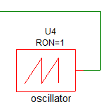
- Double click on the oscillator block to open the edit dialog. Result: The parameter editing dialog for the oscillator opens:
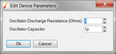
- Change the Oscillator Discharge Resistance (Ohms) parameter to 2u.
- Click Ok to save your changes.
- Press F9 to run the simulation. Notice the simulation appears slower than the previous exercise.
- When the simulation completes, select from the schematic menu. Result: The command shell displays the new time constant information.
There are 118 time constants in the .tc file
The smallest base-2 time constant is: 2^-63
Which in base-10 is approximately   : 1.08e-019
- From the SIMPLIS Status window, note the Elapsed time required to run the simulation. On the machine used to develop this example the elapsed time was 29 seconds.
Discussion: Exercise #2
In Exercise #2 you changed the oscillator discharge resistance from a realistic value of 1Ω to a value of 2uΩ which is closer to the "ideal" value of zero ohms by a factor of 500,000. However, as a consequence, you also reduced the minimum time constant for the circuit from 2-44 to 2-63, which is a factor of 219 or 524,288, which correlates well with the change in resistance. In this example circuit, the time constant formed by the oscillator discharge resistance and oscillator capacitance forms the controlling minimum time constant for the circuit. The controlling time constant determines the minimum time step which SIMPLIS takes and therefore strongly influences the elapsed time required for the simulation. Note that in this exercise, the elapsed time only changed by a factor of 3 in response to a 500000 times change in the smallest time constant. The relative ratio of elapsed time to minimum time constant is not easily predictable, as this depends on the number of energy-storage elements in the circuit, as well as the number of PWL device segments encountered during the simulation and a number of other variables. In the next exercise, you will see that for some very small circuits this controlling time constant has almost no perceptible effect on the elapsed time of the simulation.
Exercise #3: Oscillator Circuit Testbench
In this exercise you will simulate the oscillator circuit in a stand-alone testbench. You will repeat the first two exercises, and observe that the elapsed time doesn't change significantly.
- Open the schematic titled 4.5_oscillator_testbench.sxsch.
- If the SIMPLIS Status window is open, click on the Clear Message s button to clear all simulator messages.
- Press F9 to run the simulation.
- From the SIMPLIS Status window, note the Elapsed time - on the machine used to develop this example the elapsed time was 1 second.
- As in Exercise #2, change the Oscillator Discharge Resistance to 2uΩ.
- Press F9 to run the simulation.
- Again, from the SIMPLIS Status window, note the Elapsed time - on the machine used to develop this example the elapsed time was unchanged at 1 second.
Conclusion: Exercise #3
As circuit size and complexity decrease, the impact on simulation speed of a very small time constant is much reduced. Conversely, as the circuit size and complexity increase, the impact of the smallest circuit time constant becomes larger. As a model designer, you need to keep this in mind. For example, as this exercise demonstrates, a block with a very small time constant will simulate quickly when tested in a small testbench circuit. However, when this same block is integrated into a larger power supply circuit, the small time constant is dominating factor in determining the simulation time. When designing models, you need to be aware of the value of the minimum time constant of the model, and what key parameters affect this time constant. You can always check the minimum time constant for a model with the menu option used in this section.
One very helpful rule of thumb when designing SIMPLIS models is that realistic parameter values almost always result in faster simulations than "ideal" values. Realistic ON and OFF switch resistances, realistic values of Q for parasitic energy-storage elements -- realistic values in general will almost always provide better performing models than unrealistically "ideal" parameter values. There are undoubtedly exceptions to this rule, but when in doubt, it is a good place to start.
As a side note, the Voltage Controlled Oscillator (VCO) which is built-into SIMPLIS uses current sources to charge and discharge a timing capacitor; therefore, this very well thought out model doesn't suffer from small time constant issues. You can make the VCO into a fixed frequency oscillator by connecting a DC voltage source to the control pin. An example circuit using the VCO to generate the same oscillator function is provided in the download directory named 4.6_vco_testbench.sxsch. This design has a very large minimum time constant of 2-27.
Circuits With Small L/R Time Constants
The first three exercises use an example circuit with a small RC time constant. Exactly the same effect is present in circuits with a small L/R times constants. This typically occurs in transformer isolated circuits with very small leakage inductances. This problem can be solved by adding a resistor parallel to the inductor. This shunt resistor limits the high frequency response of the inductor and thereby limits the minimum time constant. SIMPLIS has a built-in multi-level lossy inductor which includes a series resistance and a shunt resistance for these applications. In the next exercise, you will see how the multi-level lossy inductor values effect the minimum time constant and the elapsed simulation time.
Exercise #4: Circuit With Small L/R Time Constants
This example circuit uses a multi-level lossy inductor for the leakage inductance, but with a very high shunt resistance of 500GΩ. The minimum time constant for this circuit is dominated by the leakage inductance divided by the resistance from the MOSFET drain to an AC ground. In this case, the parasitic resistance is the parallel combination of the MOSFET off resistance (which is 1GΩ) and the clamp diode D4 off resistance (approximately 200MegΩ). The approximate minimum time constant is therefore 100n/(200Meg) or 5E-16.
In this example you will graph the time constants as well as view the minimum time constant.
- Open the schematic titled 4.8_SelfOscillatingConverter_Slow.sxsch.
- If the SIMPLIS Status window is open, click on the Clear Messages button to clear all simulator messages.
- Press F9 to run the simulation.
- After the simulation completes, select the from the schematic menu. Result: The command shell displays the time constant information from the last simulation, and a graph of the time constants is generated.
There are 19 time constants in the .tc file
The smallest base-2 time constant is: 2^-56
Which in base-10 is approximately   : 1.39e-017
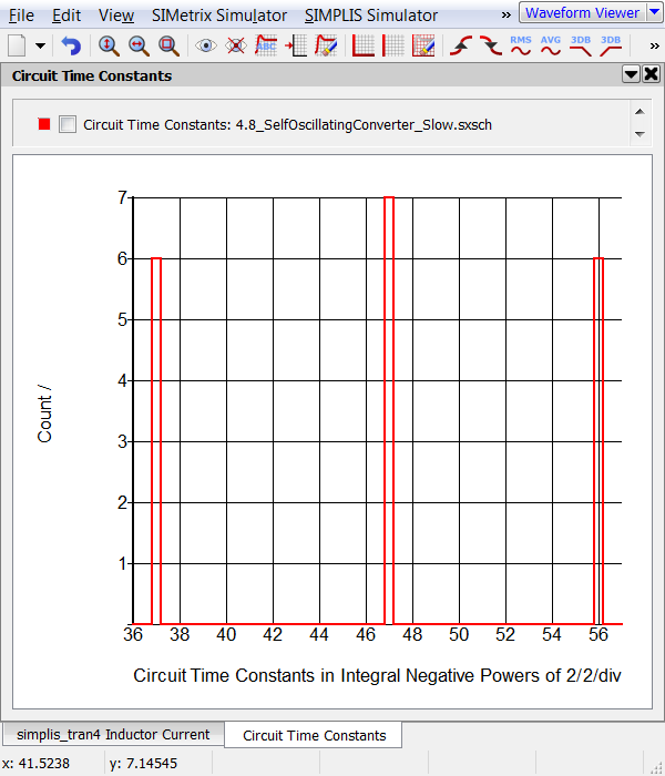 Note: This graph shows there are time constants at thee binary powers of two: 37, 47, and 56. The 2-56 time constant is the one causing the slow simulation.
 - From the SIMPLIS Status window, note the Elapsed time required to run the simulation. On the machine used to develop this example the elapsed time was 11 seconds.
- Double click on the multi-level lossy inductor Lleak, which is placed
between the MOSFET and the transformer primary winding. Result: The Edit Multi-Level Lossy Inductor dialog opens:
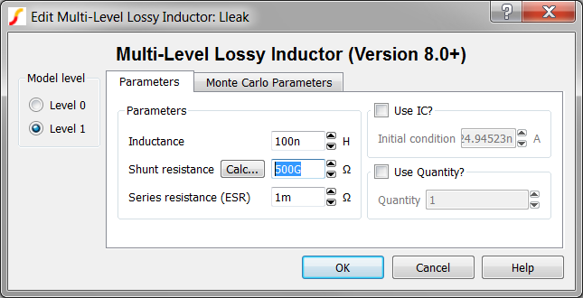 Note: The shunt resistance is 500GΩ.
 - Click on the Calc... button to calculate a new shunt resistance.Result: The Calculate New Shunt Resistance Value dialog opens.
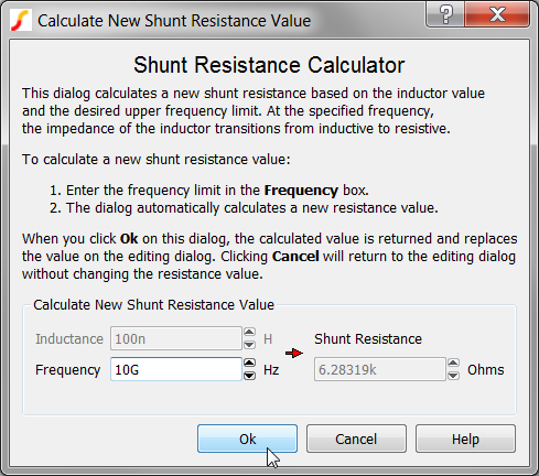 This dialog calculated a shunt resistance
based on the desired upper frequency limit. The default upper frequency limit is
10GHz, and for a 100nH inductor, the calculated shunt resistance is 6.28kΩ.
This dialog calculated a shunt resistance
based on the desired upper frequency limit. The default upper frequency limit is
10GHz, and for a 100nH inductor, the calculated shunt resistance is 6.28kΩ. - Click Ok on the Calculate New Shunt Resistance Value dialog.Result: The shunt resistance value in the main dialog is updated with the calculated value of 6.28kΩ.
- Click Ok on the Edit Multi-Level Lossy Inductor dialog.
- Press F9 to run the simulation.
- Notice the simulation runs much faster. On the machine used to develop this example, the simulation time was 2 seconds.
- After the simulation completes, select from the schematic menu. Result: The command shell displays the new time constant information from the modified circuit, and the time constant graph is updated..
There are 19 time constants in the .tc file
The smallest base-2 time constant is: 2^-41
Which in base-10 is approximately   : 4.55e-013
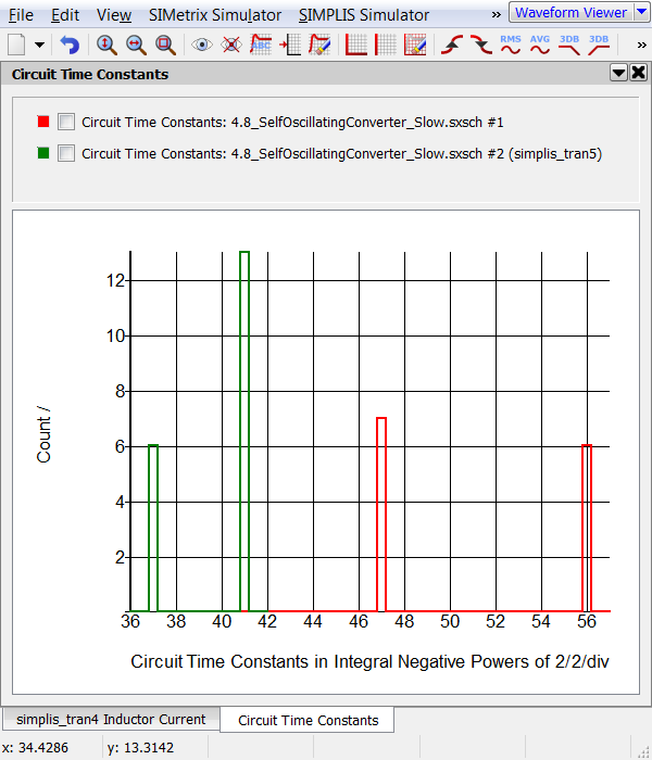
When you changed the parasitic shunt resistance to 6.28kΩ, you limited the upper frequency range of the leakage inductor to 10GHz. At frequencies above 10GHz, the inductor progressively becomes resistive with a resistance of 6.28kΩ.In the time constants graph, you see the two time constants at 2-47 and 2-56 have moved to 2-41. If you carefully examine graph, you will note there are 13 time constants at 2-41 in the second simulation, which is the sum of the first simulation's time constants at 2-47 and 2-56.
Conclusion: Exercise #4
This example illustrates a common error where modelers unintentionally create extremely small, unrealistic time constants by assuming that a more "ideal" device model will result in a better simulation result. When modeling small parasitic inductances you need to be very careful not to have unrealistically high Q parasitic inductors in series with extremely high OFF resistant switching devices.
In the original circuit, the minimum time constant was set by the multi-level lossy inductor inductance divided by the off resistance of the MOSFET. This is approximately 100n/200Meg, or 5E-16. The 500GΩ shunt resistance is too high to effect the time constant. In the second simulation, the minimum time constant is no longer set by the leakage inductance as the leakage inductance time constant is 100n/5k or 2E-11. The minimum time constant is set by another combination of circuit devices. The minimum time constant could be a RC or L/R time constant.
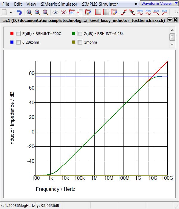
Notice the output waveforms from the two simulations are nearly identical, despite the different shunt resistance parameter values. When you changed the shunt resistance to 6.28kkΩ, you inserted a high frequency pole in the inductor impedance. As this pole is at approximately 10GHz, it has negligible effect at the frequencies present in the circuit. The image below depicts the impedance of the multi-level lossy inductor with RSHUNT=6.28k and RSHUNT=500G.
Circuits Which Rapidly Change Topologies
The oscillator circuit used in Exercise #3 changes between two topologies - a charging topology and a discharging topology. The RC time constant of the charging topology is large, as the off resistance of the switch is high. As you have seen in the previous exercises, the discharge topology controls the minimum time constant. The circuit will spend a much longer time in the charging topology than in the discharging topology.
SIMPLIS constantly observes and internally records the time duration which the circuit spends in each topology. A feature then checks the moving average of the topology time durations against a minimum time specification. If the circuit ever trips this minimum average topology duration specification, the simulator stops and an error message is generated.
In the next exercise, you will change the oscillator discharge resistance to 1uΩ and observe the error message output in the command shell.
Exercise #5: Average Topology Duration
- If you have closed the PFC example, reopen the schematic titled 4.4_PFC_Continuous_Conduction_Mode_Slow.sxsch.
- Using the same procedure as in Exercise #2, change the Oscillator Discharge Resistance. For this exercise, change the value to 1u.
- From the schematic menu, select Choose Analysis... Result: The Choose SIMPLIS Analysis dialog opens:
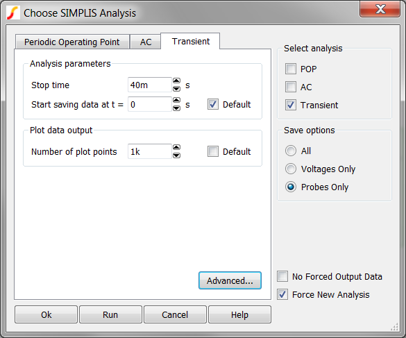
- Click on the Advanced... button to open the transient advanced options.
Result: The Transient Advanced Options dialog opens:
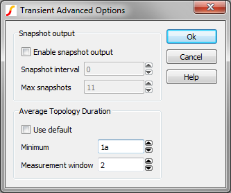
- The Average Topology Duration parameters configure the feature in SIMPLIS which
detects when circuits quickly oscillate between topologies. The operation of each
control is as follows:
Average Topology Duration Parameters
Control Description Use default Sets the Minimum to 1a (10-18), and the Measurement window to 127 topology changes. These limits will allow almost any circuit to pass the Average Topology Duration feature. Minimum The minimum time threshold which the Average Time Duration feature will allow. This time is used in conjunction with the Measurement window, which averages the time duration over a specified number of topologies. Measurement window The number of topologies used to average the time durations. This moving average computes the average time duration spent in each topology over this number of successive PWL topologies. Setting this parameter to 2 will error when a single topology whose duration is less than the Minimum specification is encountered. - Click Ok on the Transient Advanced Options dialog.
- Click Run on the Choose SIMPLIS Analysis dialog. Result: The simulation runs but stops at the first oscillator discharge state. This occurs at the simulation time of ~10us. The following error is output to the command shell:
*** ERRORS REPORTED BY SIMPLIS ***
****************************************
<<<<<<<< Error Message ID: 5049 >>>>>>>>

There were 2 topology changes in the time span from
1.0001380261689104e-005 sec. to 1.0001380261690713e-005 sec.

The averaged duration in each topology during this time
span is 8.0477394412019126e-019 sec., which is below the
default/option value of 1.0000000000000001e-018 sec.

This might be caused by unintended oscillation in the
simulation model.


*** END SIMPLIS ERROR REPORT ***
Discussion: Exercise #5
In this exercise the Average Topology Duration parameters were set to find a single PWL topology whose time duration was less than 1a (10-18) second. This well controlled experiment demonstrates one way to use the Average Topology Duration feature. The fact that a model spends a very short time in a single PWL topology does not mean the model is will simulate slowly. It is the rapid changing, or oscillating between PWL topologies which results in a slow simulation. Fortunately, real power supply circuits which display this behavior are few and far between. All examples of this behavior come from customers circuit which contain proprietary information and therefore cannot be included in this topic.
Other circuits which oscillate or "chatter" between PWL topologies include:
- Circuits with zero delay feedback loops, see 4.7_zero_delay_feedback.sxsch.
- Circuits with parallel or series combinations of PWL resistors.
SIMPLIS Debug Report Generator
Most slow simulations can be resolved using either the minimum time constant checker or the average topology duration methods. A detailed debug report for a design can be generated with the SIMPLIS Debug Report Generator. Details of how to use the debug report generator are outside the scope of this class.
Conclusions and Key Points to Remember
When you encounter a circuit which simulates slowly, the problem is usually one of the following:
- The circuit has a very small time constant.
- The circuit is oscillating between topologies.
You can troubleshoot these problems with the schematic menu items and or with the Average Topology Duration feature. If you cannot resolve the issue with these two methods, the SIMPLIS Debug Report Generator can be used.
Module Evaluation Form
Please fill out the Module # 4 Evaluation form.