6.5.2 Promoting Scalars to the Overview Report
In section 5.2 Running the Line and Load Testplan, you ran the line and load regulation testplan, which automatically included scalar values on the overview report in the CALCULATED RESULTS section. Other scalars from a test can also be copied to the overview report with the PromoteScalar() function. Any number of scalars can be promoted by using multiple PromoteScalar() calls. This function also allows you to rename the scalars.
To add scalars to an overview report, follow these steps:
- Open the testplan from
SIMPLIS_dvm_tutorial_examples.zip
at this path: testplans/6.5.1_promotegraph.testplan. Note: This is the testplan that you saved in 6.5.1 Promoting Graphs to the Overview Report.
- Insert two Promote columns after the Jumper column.
The testplan now has four Promote columns: the two that you just added plus the existing ones with the PromoteGraph() functions . An already prepared starting testplan as shown below is available from SIMPLIS_dvm_tutorial_examples.zip at this path: 6.5.2_promotescalar_start.testplan with the additional columns highlighted in red .
| *** | |||||||||
|---|---|---|---|---|---|---|---|---|---|
| *** 6.5.2_promotescalar_start.testplan: promotescalar testplan for DVM tutorial section 6.5.2 | |||||||||
| *** | |||||||||
| *?@ Analysis | Objective | Jumper | Promote | Promote | Promote | Promote | Source | Load | Label |
| *** | |||||||||
| Ac | BodePlot(OUTPUT:1) | Close(J1) | Source(INPUT:1, Nominal) | Load(OUTPUT:1, Light) | VOUT=1.505V|Bode Plot|Vin Nominal|Light Load | ||||
| Ac | BodePlot(OUTPUT:1) | Close(J1) | PromoteGraph(BODE PLOT, 100, 1, Bode Plot Nominal Vout) | PromoteGraph(LOAD, 90, 1) | Source(INPUT:1, Nominal) | Load(OUTPUT:1, 50%) | VOUT=1.505V|Bode Plot|Vin Nominal|90% Load | ||
| Ac | BodePlot(OUTPUT:1) | Close(J1) | Source(INPUT:1, Nominal) | Load(OUTPUT:1, 100%) | VOUT=1.505V|Bode Plot|Vin Nominal|100% Load | ||||
| *** | |||||||||
| *** the jumper position sets the output voltage to 0.6V | |||||||||
| *** | |||||||||
| Ac | BodePlot(OUTPUT:1) | Open(J1) | Source(INPUT:1, Maximum) | Load(OUTPUT:1, Light) | VOUT=0.6V|Bode Plot|Vin Maximum|Light Load | ||||
| Ac | BodePlot(OUTPUT:1) | Open(J1) | PromoteGraph(DVM BODE PLOT#log#ac, 80) | PromoteGraph(DVM LOAD#pop) | Source(INPUT:1, Maximum) | Load(OUTPUT:1, 50%) | VOUT=0.6V|Bode Plot|Vin Maximum|50% Load | ||
| Ac | BodePlot(OUTPUT:1) | Open(J1) | Source(INPUT:1, Maximum) | Load(OUTPUT:1, 100%) | VOUT=0.6V|Bode Plot|Vin Maximum|100% Load | ||||
Since in the last section, you promoted the Bode Plot graphs to the overview, it makes sense to also promote the scalar values for gain_margin and phase_margin from each test.
To add these PromoteScalar() entries in the first two Promote columns, follow these steps:
- Using the original scalar names of gain_margin and phase_margin, make the
following entries in the second row of the nominal output voltage scalars in the first
set of tests:
- PromoteScalar(gain_margin, Gain Margin @ 1.505V (dB))
- PromoteScalar(phase_margin, Phase Margin @ 1.505V (deg))
- To examine the the PromoteScalar() function without an overview scalar renamed, make
the following two PromoteScalar() entries in the second row of the 600mV output
voltage tests in the second set of tests.
- PromoteScalar(gain_margin, Gain Margin @ 600mV (dB))
-
PromoteScalar(phase_margin)
Note: The first entry renames the scalar and the second does not.
Result: The final testplan looks like the following, which is available from SIMPLIS_dvm_tutorial_examples.zip at this path: 6.5.2_promotescalar_final.testplan.
| *** | |||||||||
|---|---|---|---|---|---|---|---|---|---|
| *** 6.5.2_promotescalar_final.testplan: promotescalar testplan for DVM tutorial section 6.4.3 | |||||||||
| *** | |||||||||
| *?@ Analysis | Objective | Jumper | Promote | Promote | Promote | Promote | Source | Load | Label |
| *** | |||||||||
| Ac | BodePlot(OUTPUT:1) | Close(J1) | Source(INPUT:1, Nominal) | Load(OUTPUT:1, Light) | VOUT=1.505V|Bode Plot|Vin Nominal|Light Load | ||||
| Ac | BodePlot(OUTPUT:1) | Close(J1) | PromoteScalar(gain_margin, Gain Margin @ 1.505V (dB)) | PromoteScalar(phase_margin, Phase Margin @ 1.505V (deg)) | PromoteGraph( BODE PLOT, 100, 1, Bode Plot Nominal Vout ) | PromoteGraph( LOAD, 90, 1 ) | Source(INPUT:1, Nominal) | Load(OUTPUT:1, 50%) | VOUT=1.505V|Bode Plot|Vin Nominal|90% Load |
| Ac | BodePlot(OUTPUT:1) | Close(J1) | Source(INPUT:1, Nominal) | Load(OUTPUT:1, 100%) | VOUT=1.505V|Bode Plot|Vin Nominal|100% Load | ||||
| *** | |||||||||
| *** the jumper position sets the output voltage to 0.6V | |||||||||
| *** | |||||||||
| Ac | BodePlot(OUTPUT:1) | Open(J1) | Source(INPUT:1, Maximum) | Load(OUTPUT:1, Light) | VOUT=0.6V|Bode Plot|Vin Maximum|Light Load | ||||
| Ac | BodePlot(OUTPUT:1) | Open(J1) | PromoteScalar(gain_margin, Gain Margin @ 600mV (dB)) | PromoteScalar( phase_margin ) | PromoteGraph( DVM BODE PLOT#log#ac, 80 ) | PromoteGraph( DVM LOAD#pop ) | Source(INPUT:1, Maximum) | Load(OUTPUT:1, 50%) | VOUT=0.6V|Bode Plot|Vin Maximum|50% Load |
| Ac | BodePlot(OUTPUT:1) | Open(J1) | Source(INPUT:1, Maximum) | Load(OUTPUT:1, 100%) | VOUT=0.6V|Bode Plot|Vin Maximum|100% Load | ||||
To run the overview report based on this testplan, follow these steps:
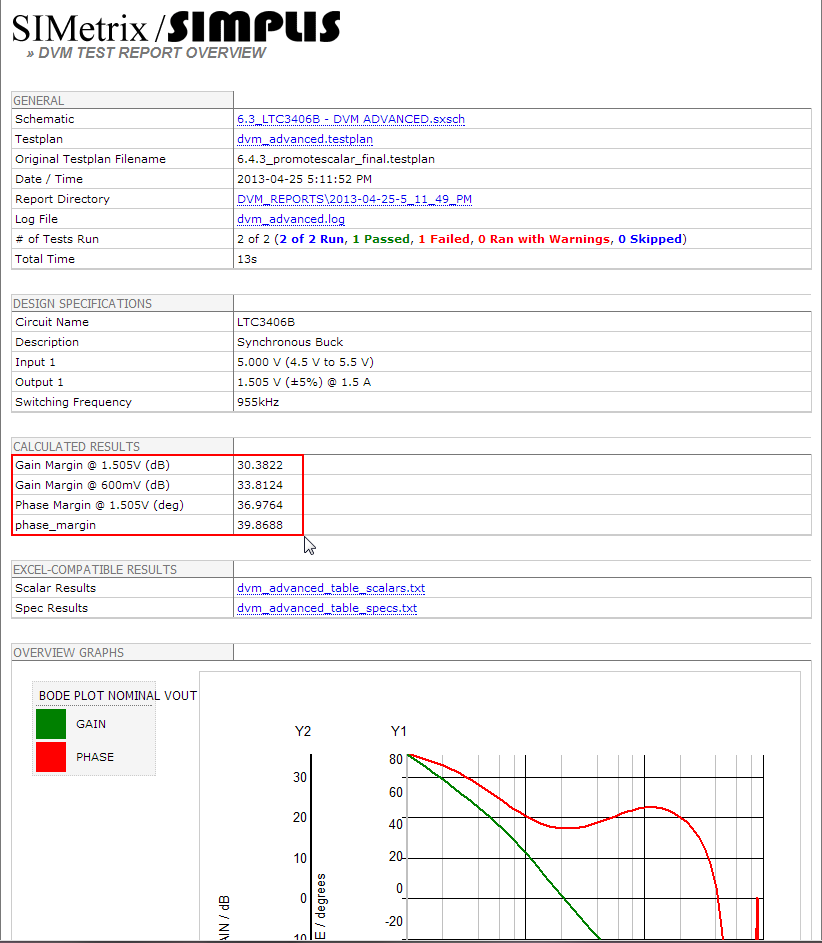
- Open the jumper schematic from section 6.3, which is available from SIMPLIS_dvm_tutorial_examples.zip at this path: LTC3406B/6.3_LTC3406B - DVM ADVANCED.sxsch.
- Run the two 50% load tests at the two different output voltages. Result: In the overview test report shown below, you can see all four scalar values with new and descriptive names for three of the scalars. The single phase_margin scalar is from the 600mV test and was not renamed. Renaming the scalars in the testplan, therefore, is another best practice to follow in order to increase the clarity of the report.