4.2 Design a Transformer in SIMPLIS MDM
In this section of the tutorial, you will design a flyback transformer for a for a 310V-to-5V, 2A output, self-oscillating converter. You will then refine that design to reduce the losses.
In this topic:
Key Concepts
This topic addresses the following key concepts:
- The structure of the transformer - the number of primary and secondary windings, their polarity, and the initial number of turns per winding - is defined before using SIMPLIS MDM, in the Windings tab of the Define Multi-Level Lossy Transformer dialog.
- The physical structure of the transformer is defined inside SIMPLIS MDM. In MDM, the number of turns can be changed, but not the number of windings and their designation as a primary or secondary winding.
- Due to the differing model structure, you can expect slightly different behaviour from a Level 3 transformer model than from a Level 2 transformer model derived from that very same Level 3 model.
What You Will Learn
In this topic, you will learn the following:
- How to design a transformer using SIMPLIS MDM
- How to analyze the results of MDM post-processing to refine your transformer design
- How to evenly space the turns of a winding layer in a transformer along the bobbin
- How to add tape between windings in your SIMPLIS MDM transformer model
4.2.1 The Self-Oscillating Flyback Converter Circuit
Open the schematic 4.2_SIMPLIS_MDM_selfoscillating_flyback_converter.sxsch from the zip archive of schematic files:
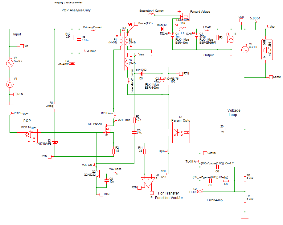
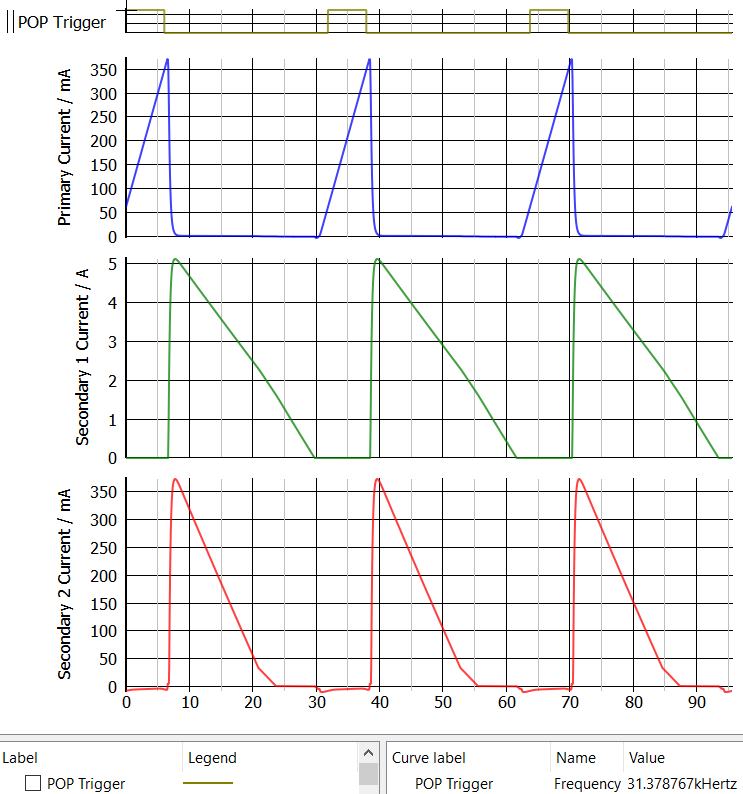
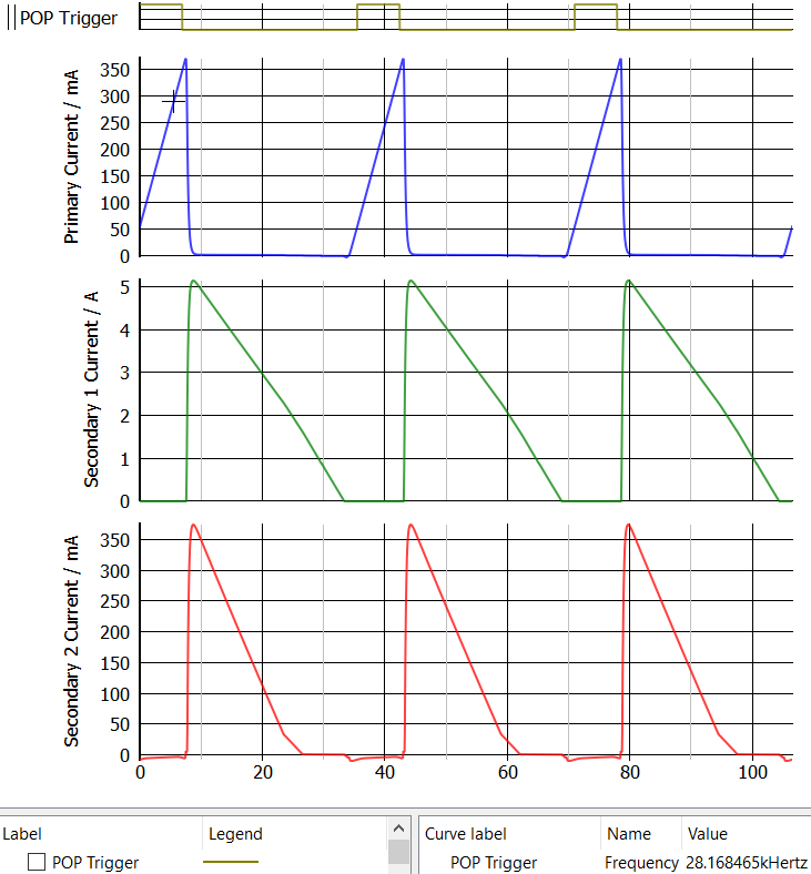
As the name suggests, this circuit does not run at a fixed switching frequency, but settles into a steady-state switching period based on the operating conditions, such as the input and output voltage and the load current. The characteristics of the transformer especially have a large effect on the steady-state switching frequency. This schematic is set up for a POP Analysis. Press F9 to run the simulation. You should see these waveforms in the waveform viewer:
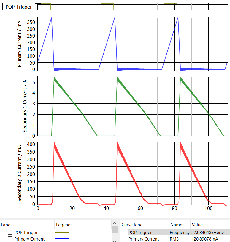
In the lower right corner you can see the frequency measurement for the POP Trigger signal, which indicates the converter's self-oscillation (switching) frequency. In this case it is approximately 27kHz. Additionally, the RMS currents for the three windings are measured, giving you an idea of the copper requirements for the windings.
In reality, selecting a transformer turns ratio and magnetizing inductance is a major part of the design of a flyback converter. However, as with the inductor examples in this tutorial, the electrical parameters and the desired turns ratios and magnetizing inductance of the transformer are taken as fixed parameters, in order to focus on building a physical model of the transformer in MDM. Therefore all the transformer designs you will create in this chapter of the tutorial will have the number of turns indicated on the transformer symbol in the schematic:
- 52 turns on the single primary winding (Primary 1),
- 3 turns on the first secondary winding (Secondary 1), and
- 7 turns on the second secondary winding (Secondary 2).
This also means that the peak current in Primary 1 will always be about 380mA, in Secondary 1 about 5.5A, and in Secondary 2 approximately 400mA, as shown in the simulation results above.
Now double-click the transformer symbol TX1 to bring up the Define Multi-Level Lossy Transformer dialog described in the previous section. You will see that the transformer is currently set to use a Level 2 model. The Level 3 model does not exist yet (which you can see by selecting the Level 3 radio button in the dialog).
Now click on the Level 0 radio button. There you will see the nominal magnetizing inductance of the transformer is approximately 6.5mH. Therefore, for all the designs in the chapter you will be targeting a magnetizing inductance of about 6.5mH. This will allow you to maintain approximately the same switching frequency as in the above simulation. Changing the magnetizing inductance significantly will have a large effect on the switching frequency.
4.2.2 Initial Transformer Design
You will now create an initial transformer design with SIMPLIS MDM using this procedure:
- In the Define Multi-Level Lossy Transformer dialog for TX1, click on Level 3 radio button.
- Click the Create Transformer Model with SIMPLIS MDM... button.Result: The main MDM window will appear, showing the Core tab:
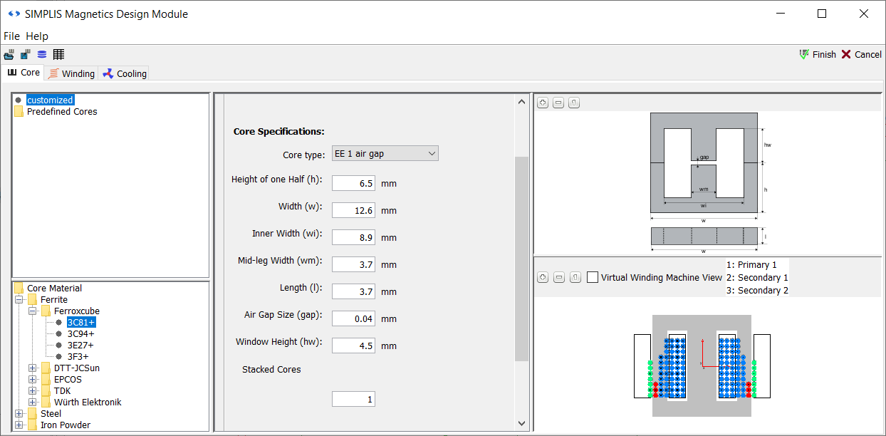
MDM has selected the first core in the database and attempted to fit the desired number of turns and monofilar windings of some default wire gauge. As you can see in the visualization to the right, the three transformer windings cannot fit into this core with the default wire size. If you attempt to click Finish right away, the MDM window will not close and you will get an error message:
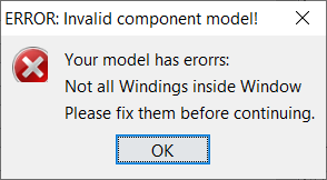
You can exit the main MDM window by clicking Finish until you have defined a physically valid design (you can of course, click Cancel to close at any time and discard your design).
Selecting a Core
The Core tab when designing a transformer works the same way as with the inductor design you completed in the previous sections. The only difference is that the number of turns (and windings) has already been defined (and placed by MDM) in the Define Multi-Level Lossy Transformer dialog. Therefore you can immediately select a core that satisfies the desired magnetizing inductance.
To start the transformer design, follow this proceedure:
- Open the MDM Status Window by clicking on the toolbar icon
 or by using the menu
File > Show status window.
or by using the menu
File > Show status window. - The core material 3C81+ should be selected by default. Change to a different material by selecting Ferrite > EPCOS > N27+.
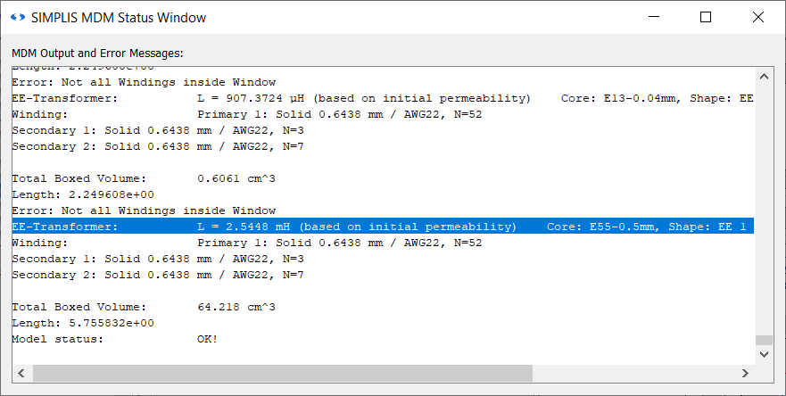
- Select the core EE 1 air gap > EPCOS > E55-0.5mm. Result: In the Status Window, you will now see a magnetizing inductance of 2.5448mH:
- The magnetizing inductance can be increased by decreasing the air gap. However, 0.5mm is the smallest air gap available in the database with EE 1 air gap cores. If you look at the Core Specifications in the center pane of the dialog, you will see that the dimensions are disabled, or grayed out, inducating that the core dimenstions are fixed. In the next step, you will switch to a custom core geometry.
- In the core geometry selection menu tree, scroll to the very top and click
customized.Result: The various Core Specifications controls are now enabled.
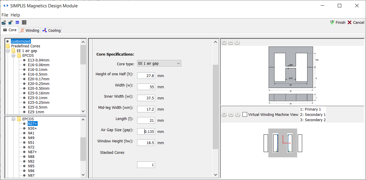
- The dimensions of the E55-0.5mm core are copied over to the customized EE 1 air gap core, and now all the dimension fields in the middle of the Core tab are editable. Scroll down until you can see the Air Gap Size (gap) field.
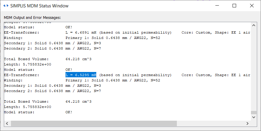
- For Air Gap Size (gap) enter 0.135 and press Enter.
Result: In the Status Window, you will now see a magnetizing inductance of 6.5295mH:
You can see that if you wish to use a customized core geometry that is not available in the database, you do not need to start by defining every core dimension from zero. You can selected the predefined core that most closely matches your requirements, and then click customized to start editing the dimensions of that core to suit your needs.
The Core tab should now appear as follows:
Designing the Windings
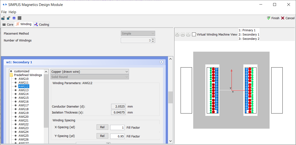
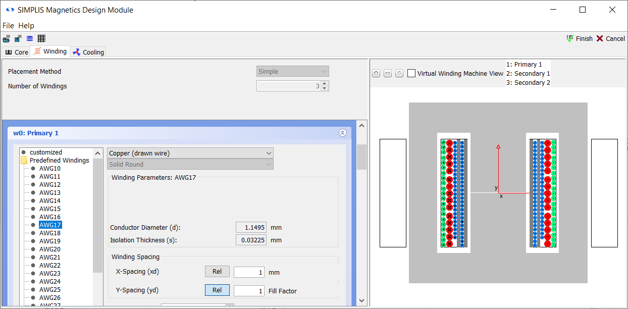
Now switch to the Winding tab of the main MDM window. You will notice some differences compared to the inductor design you did in the previous chapters:
- At the upper left is a sub-panel which defines Winding Placement and the Number of Windings. The Number of Windings is fixed to 3 and cannot be changed here since that was the number of windings defined in the Define Multi-Level Lossy Transformer dialog. The only winding placement method covered by this tutorial is the default Simple. Do not change this setting.
- The first sub-panel is for the bobbin defininition and is the same as the inductor design dialog.
- Below the bobbin sub-panel there is now a sub-panel for each transformer winding, labeled at the top with the name of the particular winding - in this case, Primary 1, Secondary 1 and Secondary 2. Each sub-panel contains the same settings to define the wire geometry and arrangement.
- Since each winding can have a different number of turns, the spinner defining the number of turns is now on each of the separate winding sub-panels, rather than at the top as in the inductor case.
- There is no Winding Pattern sub-panel as with the inductor. The Simple winding placement method covered in this tutorial is more limited in terms of the way the turns of each winding can be arranged.
The secondary windings conduct a higher RMS current (2.69A in Secondary 1 and 157mA in Secondary 2) than the primary winding (120mA). Therefore we want to devote more copper area in the winding window to the secondaries than to the primary. To design the windings for this transformer,
- Scroll to the Primary 1 sub-panel, and select the AWG17 wire.
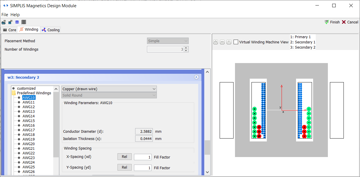
- Scroll to the Secondary 1 sub-panel, and select the largest wire available, AWG10.
- Do the same for Secondary 2, setting the wire to AWG10. Result: The Winding tab should now appear as follows:
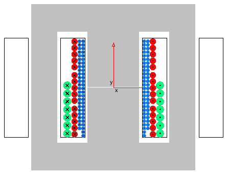
Change the Filar Count and Spacing of Secondary 1 Winding
- More copper is still required, especially for Secondary 1. The only way to do this with a standard wire size is to increase the number of wires in parallel, also known as the filarity. Scroll to the sub-panel for Secondary 1.
- In the drop-down menu next to Filar, select Y.
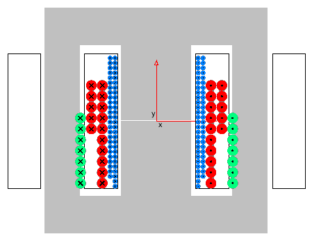
- Increase the Filar spinner to 5. Result: The three turns of Secondary 1 can now no longer fit into the winding window:
- Change the wire for Secondary 1 to AWG12. Result: All the windings now fit:

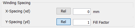
- You can space out the winding along the bobbin by changing the
parameters under Winding Spacing:
- Y-Spacing (yd) defines how much space in between each turn
is placed along the bobbin. A Fill Factor of 1 (the
default) means that the turns are just stacked right next to each other.
Change the Y-Spacing (yd) to 0.95 and press
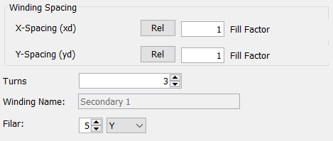
Enter. Result: Secondary 1 is now spaced evenly along the bobbin, and the three turns of 5-filar AWG12 are clearly visitble:
Change the Filar Count and Spacing of Secondary 2 Winding
- Scroll to the sub-panel for Secondary 2. Increase the Filar spinner to 3. In the drop-down menu next to Filar, select Y.
- Change the wire to AWG15.
- Change the Y-Spacing (yd) to 0.96 and press
Enter. Result: The Winding tab should now look like this:
Defining the Cooling for the Transformer
Now switch to the Cooling tab. Everything is the same as in the inductor case. Leave everything as is and click Finish.
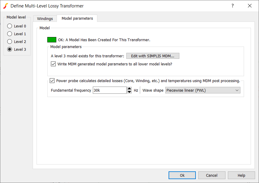
Double-click the symbol TX1. You will now see that the Level 3 model has been created:
Save the schematic as 4_myflyback_transformer1.sxch.
A complete schematic with the inductor design developed in this sub-section, set up for MDM post-processing, is available as 4.2_SIMPLIS_MDM_selfoscillating_flyback_converter_with_initial_transformer_design.sxsch in the zip archive of schematic files.4.2.3 Transformer Leakage Inductance
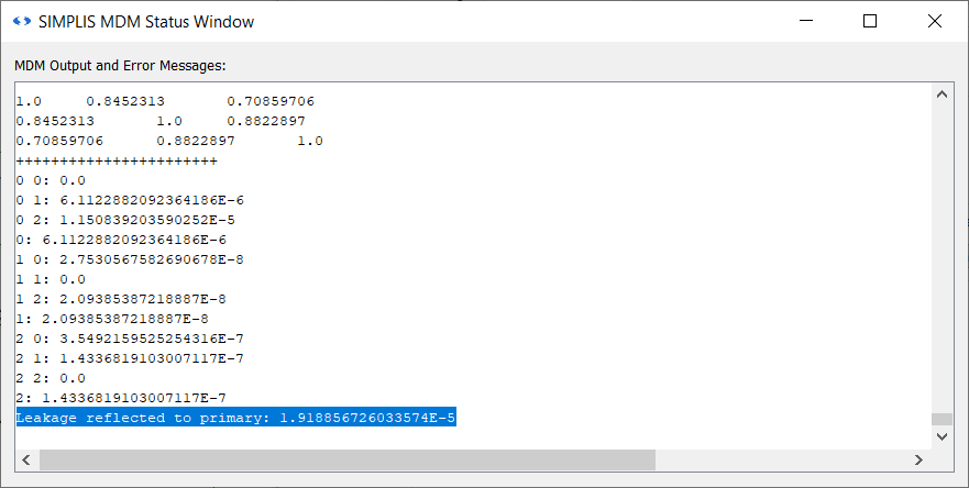
In addition to the transformer magnetizing inductance, the other important inductive property of the transformer is its leakage, or stray, inductance. Calculating the leakage inductance in MDM is a more computationally intensive process than calculating the magnetizing inductance, and therefore this value is not displayed in the Status Window every time you change a parameter of your MDM model, but is instead calculated only once you click Finish. There are two ways to then see the leakage inductance:
- The leakage inductance is displayed in the MDM Status Window after you have clicked Finish:
- You can also double-click the transformer symbol, and click the Level 2 radio button in the dialog:
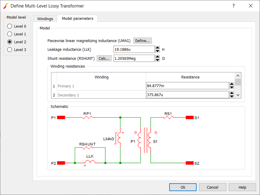
The leakage inductance will also be displayed in the MDM Results Window after MDM post-processing.
Note that in the Level 3 model, the leakage inductance is distributed throughout the reluctance circuit. It is not all lumped together and reflected to the primary as in the Level 2 model.
4.2.4 Effect of Changing Transformer Model Level
As noted in the previous section, the different transformer levels vary quite bit in their internal structure. It can be expected that this will noticeably affect the simulation results in a circuit such as this self-oscillating converter. Examine now how the result look with each different model level:
- Double-click the symbol TX1.
- Select the Level 0 model. Click OK.
- Press F9 to run the simulation.
Result: The results show an oscillation frequency of 31.38kHz.
- Double-click the symbol TX1 again.
- Select the Level 1 model. Click OK.
- Press F9 to re-run the simulation.
Result: The results show an oscillation frequency of 28.17kHz.
- Again, double-click the symbol TX1.
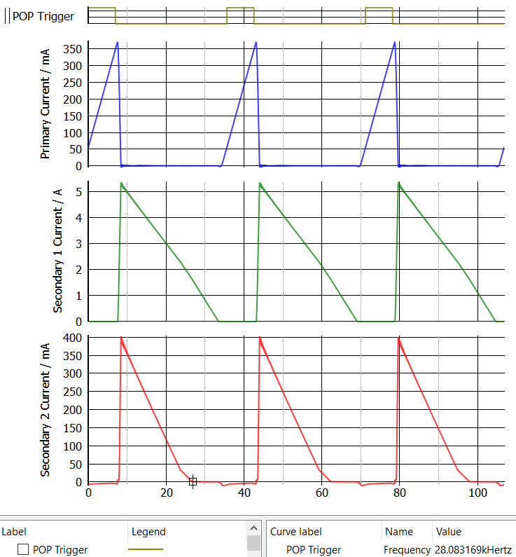
- Select the Level 2 model. Click OK.
- Press F9 to run the simulation once more.
Result: The results show an oscillation frequency of 28.08kHz.
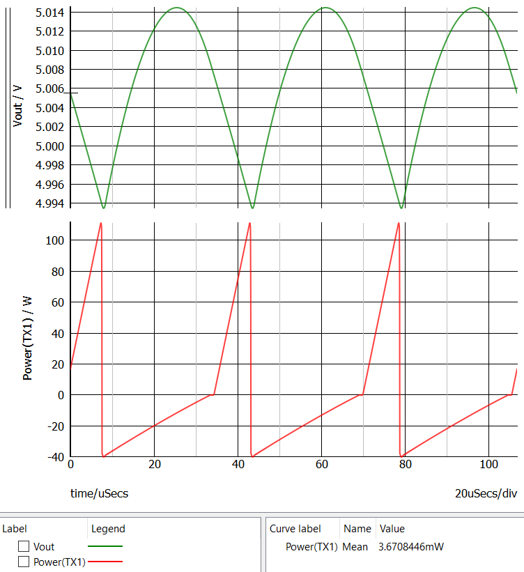
- The Level 2 model is the first to include resistive losses. Therefore click on the tab
labeled simplis_pop9 Vout at the bottom of the Waveform Viewer to
see the power loss plotted by the power probe. Result: An average loss of 3.67mW was measured in the transformer.
- Double-click the symbol TX1.
- Select the Level 3 model.
- Uncheck the Power probe calculates detailed losses... checkbox. You do not want to perform MDM post-processing on the first run of the Level 3 model.
- Click OK.
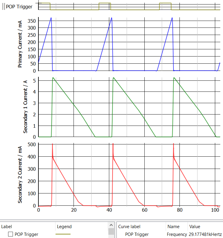
- Press F9 to run the simulation again.
Result: The results show an oscillation frequency of 29.18kHz.
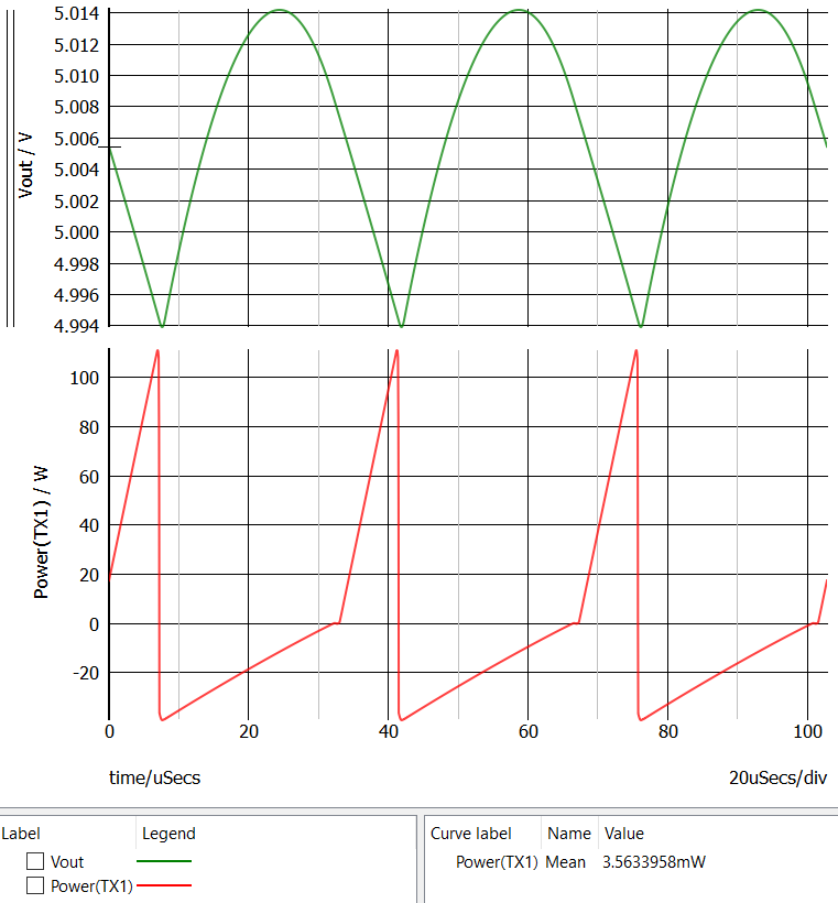
- Look at the power loss measurement by clicking the simplis_pop10 Power(TX1) tab in the Waveform Viewer.
Result: An average loss of 3.56mW was measured in the transformer.
Since the checkbox Write MDM generated model parameters to all lower level models? was checked when you created the model of this transformer in MDM, all of the model levels are consistent. The Level 3 model was created first from the physical model of the transformer in MDM, and then the Level 0, 1, and 2 models were extracted from it. Nevertheless, you can see differences in the results when simulating with each different model level. There are several things to note:
- The different structure of each model level causes the transformer waveforms to be slightly different. In the self-oscillating converter this causes the switching frequency to be slightly different in each case.
- You can see the effect of moving from a constant magnetizing inductance to a PWL one as you change from the Level 0 to the Level 1 model.
- You can see the effect of adding a leakage inductance and winding resistances as you change from the Level 1 to the Level 2 model (the PWL magnetizing inductance does not change).
- You can see the effect of using a reluctance model where the magnetizing and leakage inductances are distributed, and not just placed at the primary winding, as you change from the Level 2 to the Level 3 model (the winding resistances do not change).
- The winding resistances in the Level 2 and 3 models are the same, but the measured losses are different due to the differing current waveforms.
- The winding resistances represent the DC winding resistance only. For accurate loss results, you must run MDM post-processing.
4.2.5 Run MDM Post-Processing for the Transformer
To set up and run post-processing,
- Double-click TX1.
- Check the checkbox Power probe calculates detailed losses....
- Set the Fundamental frequency to the one identified above: 29.18k.
- Set the Wave shape to Piecewise linear (PWL).
- Click OK.
- Press F9 to run the simulation.Result: The MDM Results Window will appear once everything is complete:
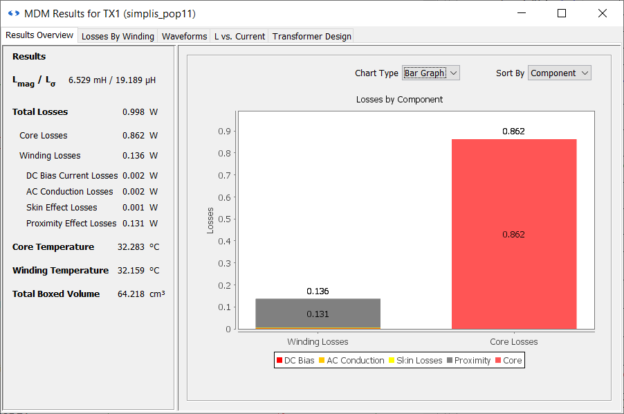
You can see that both the magnetizing inductance - 6.529mH - and the leakage inductance - 19.189μH - are displayed at the top. Also, the transformer has a boxed volume of 64.218cm3.
4.2.6 Analyze the Post-Processing Results
First of all, you can see that the transformer losses are much larger than measured previously by the power probe, with a total of 998mW! Core losses account for most of that at 862mW with winding losses being 136mW. While it's clear that previously, without the post-processing, you were not taking core losses into account, the winding losses are still about 38 times higher than measured with just the DC winding resistance. While the combined DC bias and AC conduction losses are about 4mW, similar to what was measured without post-processing, the bulk of the winding losses are actually proximity losses with 131mW. To examine why that is, switch to the Losses by Winding tab of the Results Window:
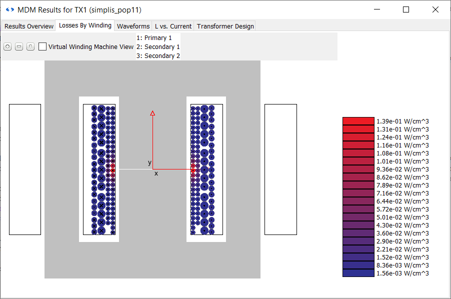
As expected, you can see some turns heating up around the air gap. However the air gap is small in this design, and it is not affecting too many turns judging from this picture. It is especially not a large influence on the losses in the secondary windings which conduct more current than the primary. It can be concluded that the proximity losses are primarily driven by the winding arrangement, i.e. are produced mainly by the fields generated by the winding turns themselves, and not the air gap.
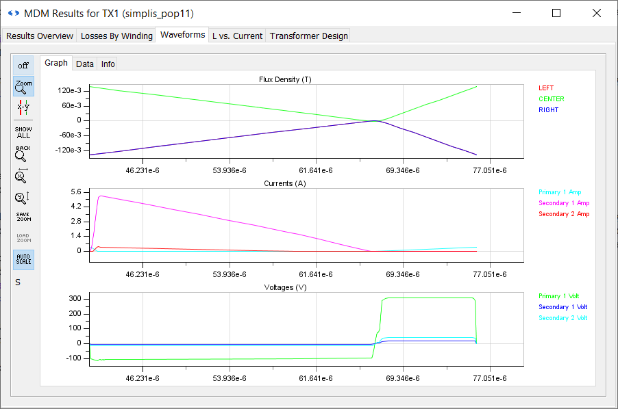
Switch to the Waveforms tab. Here, in the first plot, you can see the flux density in all three legs of the core, labeled LEFT, CENTER, and RIGHT. In the second plot the currents in each of the three windings are shown, and in the third, the winding voltages:
Magnetizing inductance as a function of current is plotted in the L vs. Current tab:
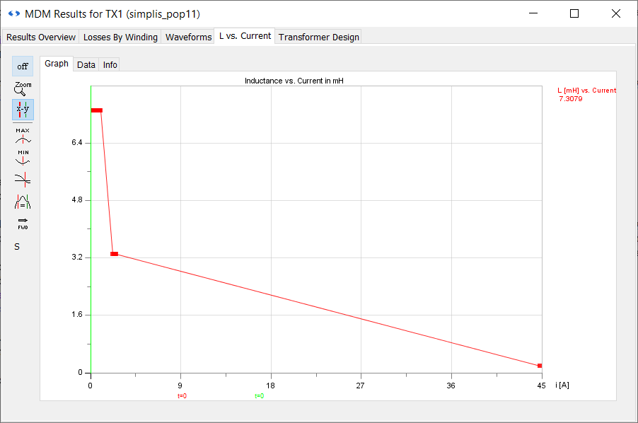
This characteristic may appear strange at first, showing that the transformer saturates rather quickly. However, note that the inductance characteristic is calculated up to the maximum flux density of the material, which in this case corresponds to a primary current of about 45A. Recall that the peak primary current in this example is much lower (less than 0.5A). To see the magnetizing inductance over the current range of interest,
- Click the
 button on the tool bar to the left of the inductance plot, to enable zooming in and out.
 - Zoom in to the part of the characteristic at the beginning of the curve by clicking your left mouse button and dragging until you create a box that spans from 0A to about 2.5A on the x-axis and approximately the full range of the y-axis.
- When you release the left mouse button, you will see a zoomed-in inductance characteristic:
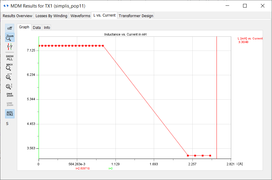
You can see now that the transformer starts to saturate above a primary winding current of about 0.95A, which is well above the peak current in this example.
4.2.7 Refine the Transformer Design
Now you will refine the design of the transformer to reduce the proximity losses. To do so,
- Double-click the symbol TX1.
- Click the Edit with SIMPLIS MDM... button.
- In the main MDM window, go to the Winding tab.
- The first thing you can do to reduce the proximity losses is to add tape in between the bobbin and the primary winding, to move the wire away from the air gap. Adding tape in between the two layers of the primary winding will both move the second layer further away, and separate the layers, reducing the effect of their proximity fields on one another. Tape is added by modifying the X-Spacing (xd) parameter. Locate it on the panel for Primary 1.
- Click the Rel button next to X-Spacing (xd). This changes the spacing definition from Fill Factor to mm:
- Now you can enter an absolute spacing - a tape thickness - in millimetres. For X-Spacing (xd), enter 1 and press Enter.
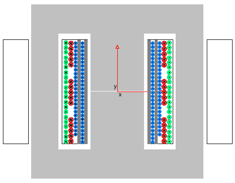
Result: Tape is now drawn in between the bobbin and Primary 1, and in between the two layers of Primary 1:
- To reduce the proximity losses in the secondary windings, change them from solid to litz wire. Scroll down to the sub-panel for Secondary 1.
- In the right wire selection menu tree, select the PF AWG38 135 wire. This indicates 135 strands of AWG38 wire per turn.
- Since you have reduced the total diameter of the wire by doing this, to spread out the turns along the bobbin change the Y-Spacing (yd) to 0.7.
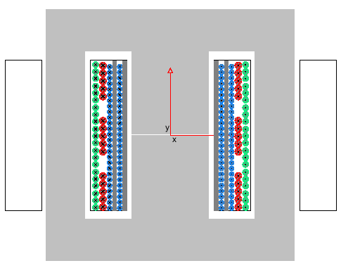
Result: Secondary 1 will now be redrawn:
- Scroll down to the sub-panel for Secondary 2.
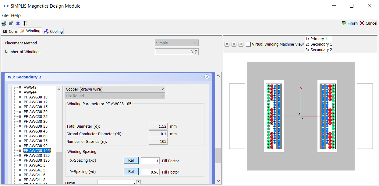
- Change the wire to PF AWG38 105.
Result: Secondary 2 will now be redrawn:
- Click Finish
- Press F9 to run the simulation.
Result: The MDM Results Window pops up:
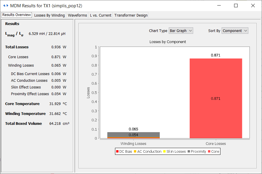
- You will see in the Waveform Viewer that the switching frequency has changed slightly to 29.16kHz. Although the magnetizing inductance is the same, the leakage is now different at 22.814μH, and this has affected the frequency. The DC winding resistances in the circuit have also changed. The losses have been reduced to 936mW, and the proximity losses have been more than halved to 54mW. Now see if they can be reduced even more by changing the primary winding to litz wire as well.
- Double-click TX1.
- Click the Edit with SIMPLIS MDM... button.
- Go the Winding tab in the main MDM window and change Primary 1 to use the PF AWG41 135 wire.
Result: Primary 1 is redrawn:
- Click Finish.
- Press F9 to run the simulation.Result: A new MDM Results Window pops up:
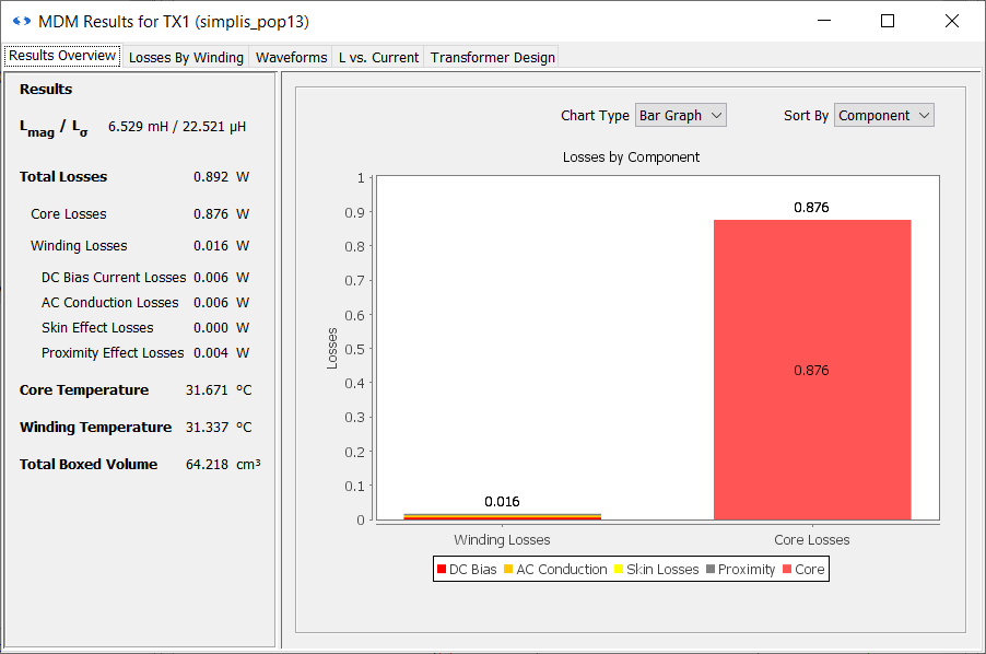
The losses are now reduced even further, and compared to the initial design are by slightly more than 10% to 892mW. Winding losses have been reduced to 16mW and proximity losses are only 4mW! DC and AC conduction losses are larger due to the smaller total wire diameters used compared to the initial design, but this is more than compensated by the drop in proximity losses.
Switch to the Losses By Winding tab:
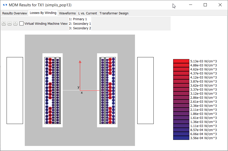
You can see almost no effect of the air gap on the winding losses here. Also, Secondary 1 is the reddest - because it conducts the highest current. The loss distribution is now driven by the conduction loss, not the proximity loss as was the case previously.
The changes made to the design have however not reduced the core losses. You will change to a design with much lower core losses in the next section.
Save the schematic as 4_myflyback_transformer2.sxch.
A complete schematic with the inductor design developed in this sub-section, set up for MDM post-processing, is available as 4.2_SIMPLIS_MDM_selfoscillating_flyback_converter_with_refined_transformer_design.sxsch in the zip archive of schematic files.