Creating Models
In this topic:
Overview
SIMetrix provides a soft recovery diode model for use in power electronics circuits. As this model is not a SPICE standard, there are no models available from device manufacturers or other sources. So, we therefore also developed a soft recovery diode "parameter extractor" that allows the creation of soft recovery diode models from data sheet values.
The parameter extraction tool works directly within the schematic environment and may be used in a similar manner to other parameterised devices such as the parameterised opamp. However, there is also an option to save a particular model to the device library and so making it available as a standard part.
In addition, SIMetrix offers a tool for creating a saturating inductor model from a data sheet Inductance vs Current curve.
Creating Soft Recovery Diode Models
-
Select menu
You will see this dialog box:
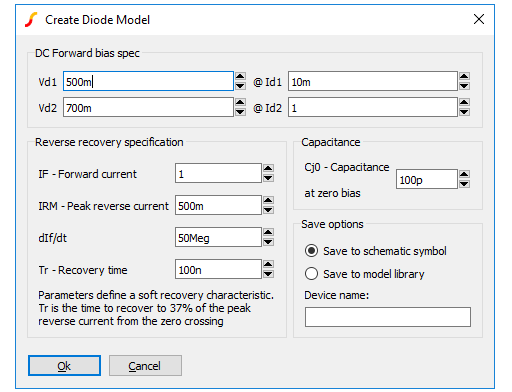
- Enter the required specification in the DC Forward bias spec, Reverse recovery specification and Capacitance sections. See below for technical details of these specifications.
- Select Save to schematic symbol if you wish to store the specification and model parameters on the schematic symbol. This will allow to you to modify the specification later. If you select Save to model library, then the definition will be written to a library file and installed in the parts library. This will make the new model available as a standard part, but you will not be able to subsequently modify it other than by re-entering the specification manually. If you choose this option, you must specify a device name in the box below.
- Click Ok to place diode on the schematic. If you selected Save to model library, the model file for the device will also be created at this point. The file will be saved in your user models directory. This is located at "My Documents\SIMetrix\Models".
Soft Recovery Diode Specification
The parameter extractor allows the specification of three important characteristics of the diode. These are the DC forward bias voltage, reverse recovery and capacitance. Currently, reverse leakage and breakdown characteristics are not modelled.
To specify the forward bias characteristics, simply enter the coordinates of two points on the graph showing forward drop versus diode current which is found in most data sheets. You should choose values at the extremes. The low current value will essentially determine the value of the IS parameter while the high current value defines the series resistance of the device.
The reverse recovery characteristics are explained in the following diagram.
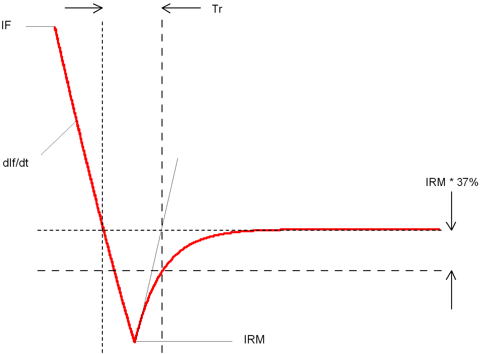
The values quoted in data sheets vary between manufacturers. The value given for Tr is sometimes taken from the reverse peak rather than the zero crossing. If this is the case you can calculate the time from the zero crossing to the reverse peak using the values for IRM and dIf/dt and so arrive at the value of Tr as shown above.
Some data sheets do not give the value of IRM. In these cases the best that can be done is to enter an intelligent guess.
Capacitance is the measured value at zero bias. Unfortunately this is not always quoted in data sheets in which case you can either enter zero (which may speed simulation times) or enter an estimated value. Of course an alternative would be to measure the capacitance of an actual device.
Notes of Soft Recovery Diode Model
The soft recovery diode does not use the standard SPICE model but a model based on work at the University of Washington. Full details of the model can be found in the Simulator Reference Manual.
Creating Power Inductor Models
- Saturation
- Series and shunt resistance
Saturation effects are entered as a lookup table and may optionally be defined by digitising a graph image.
For technical details about the underlying simulation model please refer to Simulator Reference Manual/Analog Device Reference/Inductor (Table lookup)
Power Inductor Specification
To create a power inductor model, select menu . This will show the following dialog box:
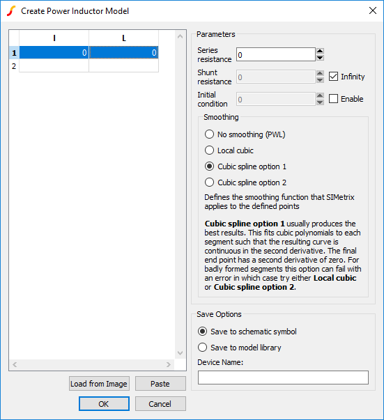
The various elements of the dialog box are explained below
| Dialog element | Description | ||||||||
| IL Table | Table of values that defines the inductance vs current. The table should only define a single quadrant; the power inductor model implementation will automatically generate inductance values for negative current. You can enter these values manually, paste the values from an external source or you can digitise a graph image. To digitise a graph image, click on Load From Image. This will invoke the data sheet curve digitiser. See Digitising Data Sheet Curves. When complete the data from the data sheet curve digitiser will be entered into the IL Table. | ||||||||
| Series resistance | Series resistance of the inductor | ||||||||
| Shunt resistance | Parallel resistance applied across the inductor | ||||||||
| Initial condition | If enabled the inductor will behave like a current source during the DC operating point calculation with the current specified here. If disabled the inductor will be a short circuit during the operating point calculation | ||||||||
| Smoothing |
Sets the smoothing function of the inductor model. The points entered in the IL Table may optionally be smoothed using a mathematical function. Options are:
|
||||||||
| Save options | Use Save to schematic symbol to save model parameters directly on the schematic symbol. Use Save to model library and enter a model name to save a model in the model library. This will be available to be placed in other schematics using the menu . Note that you will not be able to make subsequent edits to the model if using this option. |
Digitising Data Sheet Curves
The graph data extraction tool can be used to extract values from datasheet curves that can be imported for use within models in Pro and Elite versions of SIMetrix and SIMetrix/SIMPLIS. One such use is in the Power Inductor Model. It also available as free-standing tool to digitise any graph found in an image file. The free standing version can be initiated using the schematic menu or directly with the script command GraphImageCapture.
To use the tool, first an image of a graph is required. These graphs will often come from manufacturer data sheets or websites. In some cases you may be able to copy the images direct from the website or you may need to use a screen capture from a PDF image and save that image to file. The tool supports images in PNG, JPG, BMP and GIF formats, where PNG is the preferred format.
Image Requirements
The tool is designed to handle many different layouts of graphs and quality of images. The tool can accept graphs with:
- Single or multiple plotted data series
- Linear or logarithmic axes
- Grid marker lines
- Poor quality text (text labels are not required for the tool to operate)
- Graphs on light or dark backgrounds
The tool will perform poorly and may fail to give reasonable values for graphs that are at an angle.
Step 1: Grid and Boundary Detection
The first step of the tool is to determine the boundary of the graph along with any grid lines. For this demonstration, we will use the following image:
 |
The graph we want to capture data from, with grid lines and a single data series. |
When the image is loaded, the tool will make an initial estimate of where the graph bounds are and any grid lines there might be. The bounds will be highlighted in blue, whilst the grid lines will be highlighted in red, as shown in the next figure.
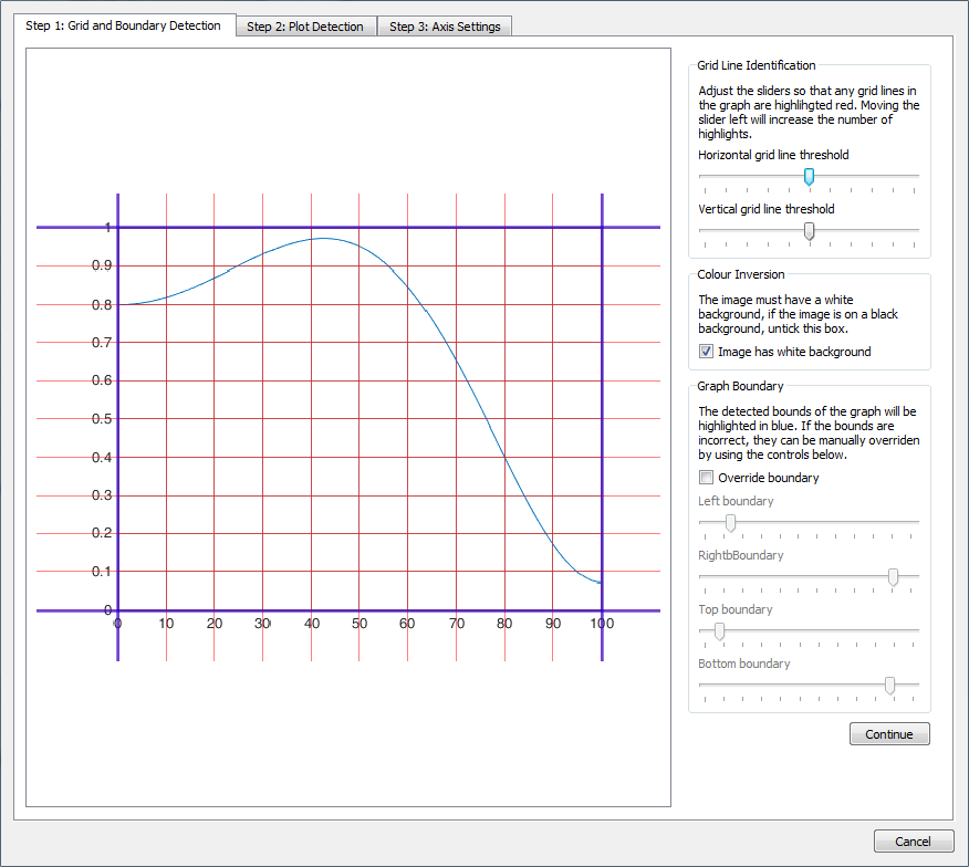 |
View of the first step window after the example image is first loaded. |
In many cases no action on the users part will be required in Step 1. Before continuing to step 2, ensure that the boundary of the graph is highlighted in blue, as many grid lines as possible are highlighted red and that if the image is on a black background, the colour inversion tick box is unchecked. Of these requirements, ensuring the bounds of the graph are correct is the most important as this is used by the final data point extraction. Getting the grid lines fully identified is not essential, this just makes the user interaction in step 2 easier. To make adjustments to the boundary and grid line identification, there are a number of sliders to the right of the window.
For Grid Line Identification, you can control how sensitive the selection of grid lines are in the horizontal and vertical plane. By moving the sliders the to left, their selection becomes more sensitive and a greater number of lines will be detected, whilst moving to the right will cause less grid lines to be identified. Adjusting these sensitivity bars can lead to grid lines not being detected or false detections from occurring.
For Graph Boundary, you control the position of the boundary lines and consequently the region of interest within the graph. This can be useful for not only correcting issues where the boundary detection has failed, but also for restricting the part of the graph that you are interested in generating data from if you only want to extract data from part of a graph.
Note: If there are lines not displaying, try resizing the window horizontally as due to image compression in displaying the resulting images.
Once this step is complete, press Continue.
Step 2: Plot Detection
The second step is to pick out the curve that you want to extract the data from. If any grid lines were all successfully detected and the bounds set, you will begin with a preview similar to that shown in the next figure.
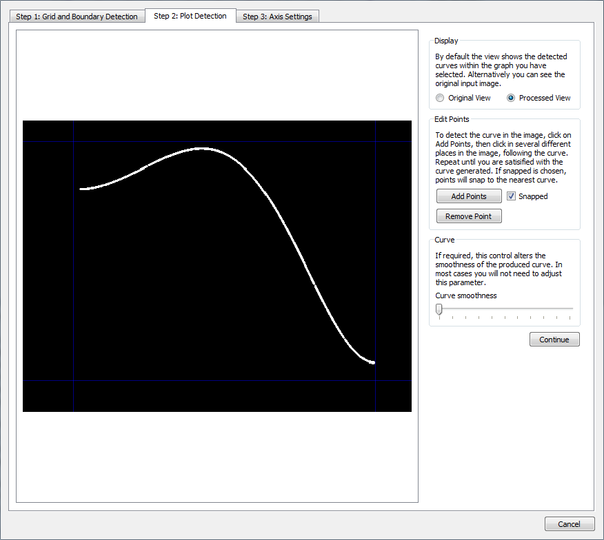 |
View of the second step window after completing step 1. Currently no curve has been marked out for use. |
To mark out the curve to use, press the button Add Points and click along the line you want to use, a red square will be placed for each point added. By default the points will snap to the curve nearest where you have clicked, so you should not need to be highly precise in where you click. To disable the snapping behaviour, uncheck the Snapped check box. As you add points, a red line will preview the line that will be used to generate data from, as shown in the next figure. This red line will not snap to a curve, because although the solution may look obvious for full automatic-detection in the single line case presented, in cases where there are multiple lines of the image is of a lower quality, such automation would be highly error prone. Instead, after adding a few initial points, add further points in places where the red line does not match the curve you want to capture.
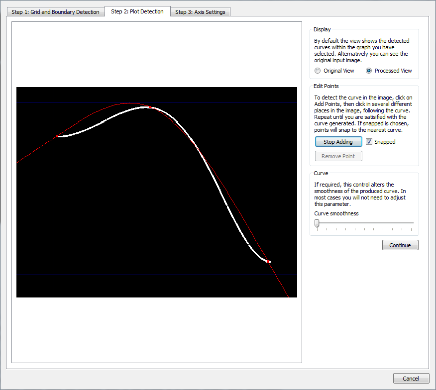 |
Line detection after three points have been added. The red line shows the line that data will be obtained from in the final step. This line does not currently match the actual curve that was on the graph shown in white, meaning further points are required to be added in places where the curves do not match. |
Generally you will not require many points to be placed to obtain a red line that well resembles the curve you want to capture. As shown in the next figure, you many not need to place many points along regions of the graph with consistent behaviour, such as continuous curves or straight regions. In areas where greater precision is required, you may require several closely positioned points.
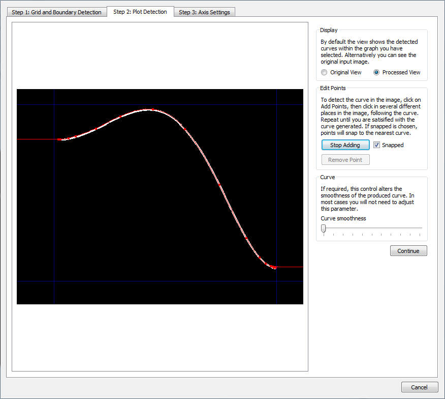 |
A completed line detection. Points are spaced out for the majority of the curve but are more dense at the ends of the curve due to the curve levelling out at those regions. |
If a point is added erroneously, press the Stop Adding button then press the Remove Point button and click on the point you want to remove. The remove point behaviour only works for one point at a time. If multiple points are to be removed, the Remove Point button will need to be pressed each time.
Whilst the curves produced by this method should generally provide a good representation through simply adding points alone, there may be situations where the red curve generated is not smooth enough to fit those points. In these cases the Curve smoothness slider can be used to make the curve smoother. For most usage the slider can remain in the it's default position of fully to the left. Moving the slider fully to the right will make the curve become more smooth and with the slider fully to the right the curve will become a straight line.
When the curve detection is complete, press continue.
Step 3: Axis Settings
Now that the bounds of the graph and a curve has been selected, the final step is to determine the values of the axes. As shown in the next figure, the final step will show the originally loaded graph image, along with the graph bounds highlighted in blue and the selected curve in red. If either the bounds or curve do not appear to be correct, you can go back to the previous stages and update them.
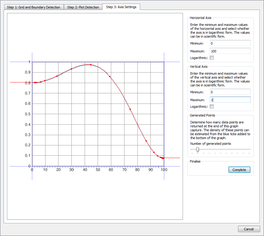 |
A completed line detection. Points are spaced out for the majority of the curve but are more dense at the ends of the curve due to the curve levelling out at those regions. |
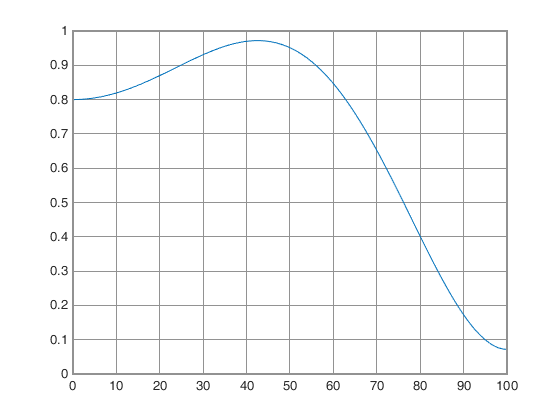
To submit values for the axes, set the minimum and maximum values for the graph bounds in the text boxes to the right of the graph image. In this example the minimum value on the horizontal axis is at 0, with maximum at 100. For the vertical we have minimum of 0 and maximum of 1. If either of the graphs are a logarithmic axis, select the logarithmic scale check box.
Finally you can determine the granularity of the points generated by adjusting the Generated Points slider. Moving the slider to the left increases the number of points. An indication of where the samples will be taken from can be seen by the blue ticks on the horizontal axis.
When all stages are complete, press the Complete button. If the button is disabled, messages will appear stating what stages have not been completed that are required. When the Complete button is pressed, the dialog will return vectors of data points that have been extracted from the curve.
| ◄ Generic Digital Parts | Subcircuits ▶ |