1.0.5 POP and AC Analysis
The Periodic Operating Point (POP) analysis is one of the most powerful capabilities of SIMPLIS. The POP analysis is a specialized transient analysis which quickly finds the switching steady-state operating point of a circuit. Once the steady-state operating point is found, an AC analysis at the periodic operating point can be performed on the circuit.
The POP analysis can also be followed with a transient analysis, in which case the transient simulation will start at the operating point found in the POP analysis. This is very useful for tests such as a pulse load transient where the circuit starts in steady-state.
In this topic:
Key Concepts
This topic addresses the following key concepts:
- The Periodic Operating Point (POP) analysis is a specialized transient analysis.
- The POP analysis literally forces the circuit into a steady-state condition by putting an extra control loop around the converter.
- The POP analysis solves the steady-state operating point to a high level of precision, much higher than the RELTOL of a SPICE simulator.
- A successful POP analysis is required to run an AC analysis.
- SIMPLIS looks at your circuit in terms of topologies, or unique circuit configurations.
- The AC analysis results are valid at the switching operating point found in the POP analysis.
What You Will Learn
In this topic, you will learn the following:
- The basics of how a SIMPLIS Periodic Operating Point analysis works.
- Why POP is so important when simulating switching power circuits.
- What a new topology is.
Getting Started: Running a POP and AC Analysis
- If the waveform viewer is open, close it.
- If the SIMPLIS Status window is open, select the window (Ctrl+Space), and click the Clear Messages button to clear all messages from the window.
- Open the schematic titled 1.2_SIMPLIS_tutorial_buck_converter.sxsch.
- From the menu bar select .
- Un-check the Transient checkbox, leaving the POP and AC
analysis checkboxes checked.Result: The POP Checkbox is also checked, but disabled - indicating you must run a POP analysis before every AC analysis.
- The dialog should appear as follows:
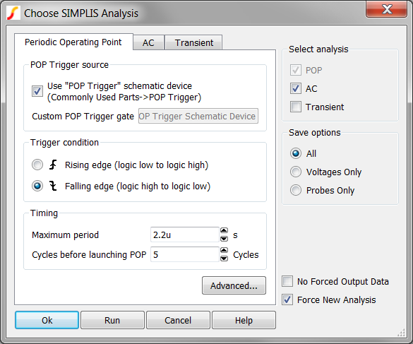
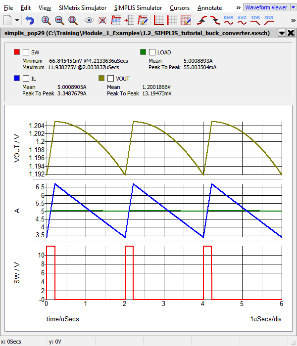
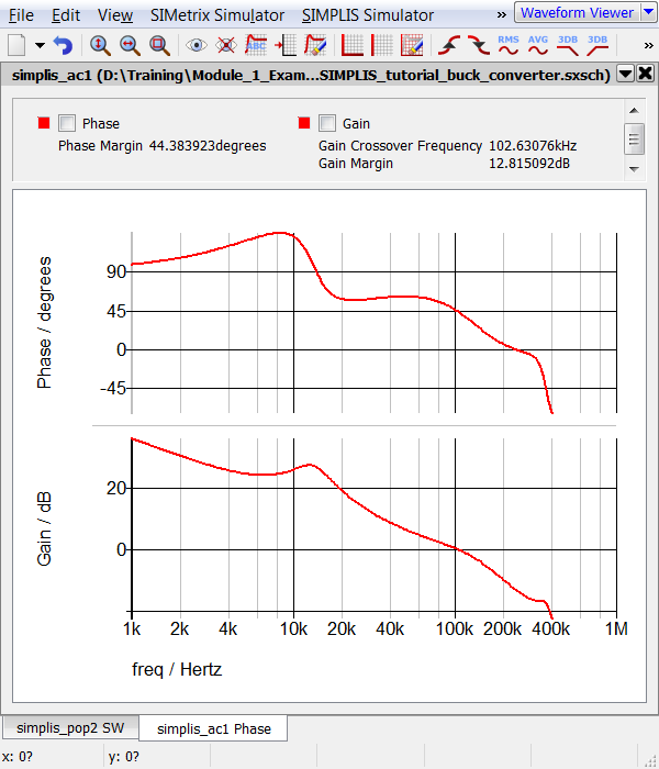
- Click Run. Result: The POP analysis runs on the Synchronous Buck Converter, finding the switching steady-state operating point of the circuit and then runs the AC analysis. The waveform viewer opens with 3 switching cycles of data along with the AC response of the control loop.
Discussion - POP Analysis
When you go into the lab and power up a switching power circuit, it has several seconds to settle into steady state before you view or capture your first oscilloscope image. Even the slowest PFC control loop with a bandwidth of a few Hertz will settle in the time between when you power up the circuit and when you first probe the circuit. Life in the simulator is a little bit different - we need a way to accelerate the time required to get to steady-state. This is exactly why the Periodic Operating Point was developed.
How POP Works
POP is essentially a software control loop around your power supply control loop. POP monitors each switching cycle of the converter. The POP Trigger device detects a waveform edge signaling the beginning of the next switching cycle, much like the oscilloscope trigger captures waveforms in the lab. At each edge, the POP algorithm takes a number of actions:
- Samples and records each capacitor voltage and each inductor current.
- Records the current operating segment of each PWL device, whether that device is a resistor, capacitor, or inductor.
- Records the state of each switch in the circuit.
Armed with this information, POP then simulates the circuit for another switching cycle. POP then re-samples the capacitor voltages and inductor currents, and makes a calculation to determine if the values are essentially the same from one switching edge to the next switching edge. If the percent error is less than the POP convergence specification, the POP algorithm decides the converter is in steady state and exits. The simulation time is reset to zero, and a user specified number of switching cycles, three in this case, are simulated and plotted on the waveform viewer.
What if the sampled values from one switching edge to the next are greater than the convergence specification? POP will take another pass through the loop, during each pass:
- POP will predict what the capacitor voltages and inductor currents should be for the converter to be in a steady-state condition.
- POP loads the circuit with these initial conditions and re-starts the simulation.
- At the next switching edge, the process repeats.
SIMPLIS Status Window Displays POP Progress
- The percentage completion for each analysis.
- Elapsed and CPU times for each analysis.
- The POP convergence found for each pass through the POP process.
- New topology information. A new topology is a unique circuit configuration, for example, in this buck converter, there is a new topology when the MOSFET turns on, and another when the MOSFET turns off. You will learn more about new topologies in section 2.0 Transient Analysis Settings.
The SIMPLIS Status window offers a peek into how the POP algorithm works. Shown below is the output from the POP simulation run.You can view the status window text as a file in a new browser window by clicking 1.0.5_simplis_status_window_pop_analysis.log:
               ********************************************************************************
               ********************************************************************************
               simplis VERSION 8.10, RELEASE Rel-17.10.3, Mar 21, 2017
               Checking syntax of ``1.2_SIMPLIS_tutorial_buck_converter.deck''

               New topology #1
               New topology #2
               New topology #3
               New topology #4
               New topology #5
               New topology #6

               A starting operating point located.
               Elapsed time   :  0 hr  0 min  1    sec
               CPU time       :  0 hr  0 min  0.06 sec
               Simulation time: 0.000000000000e+000 sec


               PERIODIC OPERATING-POINT ANALYSIS


               New topology #7
               New topology #8
               New topology #9
               New topology #10
               New topology #11
               New topology #12
               New topology #13
               New topology #14
               New topology #15
               New topology #16
               New topology #17
               New topology #18
               New topology #19
               New topology #20
               New topology #21
               New topology #22
               New topology #23
               New topology #24
               New topology #25
               New topology #26
               New topology #27
               New topology #28
               New topology #29
               PASS   1: 6.868701e+000 %
               New topology #30
               New topology #31
               New topology #32
               New topology #33
               New topology #34
               New topology #35
               New topology #36
               New topology #37
               New topology #38
               New topology #39
               New topology #40
               New topology #41
               New topology #42
               New topology #43
               New topology #44
               New topology #45
               New topology #46
               PASS   2: 5.504316e+000 %
               New topology #47
               New topology #48
               New topology #49
               New topology #50
               New topology #51
               PASS   3: 2.494227e+000 %
               New topology #52
               PASS   4: 3.855308e-002 %
               PASS   5: 1.430737e-005 %
               PASS   6: 2.455660e-013 %
               Elapsed time   :  0 hr  0 min  1    sec
               CPU time       :  0 hr  0 min  0.04 sec
               Simulation time: 0.000000000000e+000 sec


               01 02 03 04 05 06 07 08 09 10
               11 12 13 14 15 16 17 18 19 20
               21 22 23 24 25 26 27 28 29 30
               31 32 33 34 35 36 37 38 39 40
               41 42 43 44 45 46 47 48 49 50
               51 52 53 54 55 56 57 58 59 60
               61 62 63 64 65 66 67 68 69 70
               71 72 73 74 75 76 77 78 79 80
               81 82 83 84 85 86 87 88 89 90
               91 92 93 94 95 96 97 98 99 100
               Elapsed time   :  0 hr  0 min  1    sec
               CPU time       :  0 hr  0 min  0.09 sec
               Simulation time: 6.000000000000e-006 sec


               Writing pertinent data files ...
               Leaving SIMPLIS.
After each pass through the POP algorithm, the pass number and the measured convergence is output to the SIMPLIS Status Window. Each pass is a complete loop through the POP algorithm as described above. The final convergence for this circuit is 2.45E-13%. SIMPLIS routinely solves circuits to this level of accuracy, which as you will see in the next section, allows you to run an AC analysis on the time-domain model.
This topic is an overview of the POP analysis. You will learn the details of the POP algorithm in 2.2 How POP Really Works.
Discussion - AC Analysis
As described in 1.0.1 SIMPLIS is a Time-Domain Simulator, all the Time, for Every Analysis, Period, the AC analysis is carried out on the time domain model by first finding the Periodic Operating Point, then injecting a single time-domain sinusoidal perturbation signal into the circuit. The AC results are then calculated from the time domain response to the perturbation signal. Then the injected signal is stepped to the next frequency to be analyzed and the measurement process is repeated until the entire requested frequency range is covered. No averaged model is used. All AC analysis results are derived from the time-domain response of the full nonlinear system.
What Can Go Wrong?
- If the circuit does not POP successfully, in other words, if SIMPLIS cannot find a stable steady-state periodic operating point, the AC analysis will not be run. A warning message appears in the command shell.
- Your circuit may converge during the POP analysis, but to a periodic operating point which you are not expecting. A common example occurs when the POP analysis results in the circuit operating in a current limit or other fault condition. Since during current limit operation, the voltage loop is essentially open, the gain of the voltage loop is greatly attenuated compared to what it would be in normal operation..
Conclusions and Key Points to Remember
- The reduction in time to reach steady-state using the POP analysis greatly reduces the time required in the design iteration process.
- The POP algorithm only works if the circuit is switching in a periodic fashion.
- The SIMPLIS PWL circuit equations are solved to a very high degree of accuracy. The POP convergence spec is many orders of magnitude smaller than the relative tolerance (RELTOL) of a SPICE simulator.
- Every AC analysis must be preceded by a POP analysis.
- The AC results are totally and completely dependent on the operating point found during the POP analysis.