2.4.4 Plotting Frequency Spectrums
To download the examples for Module 2, click Module_2_Examples.zip
In this topic:
What You Will Learn
- How to plot the Frequency Spectrum of a voltage or current.
- How to use the Spectrum() function to plot Frequency Spectrums.
Getting Started
Exercise #1: The Define Fourier Plot Dialog
- Open the schematic 2.5_SelfOscillatingConverter_POP.sxsch.
- Run the simulation.
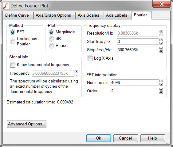
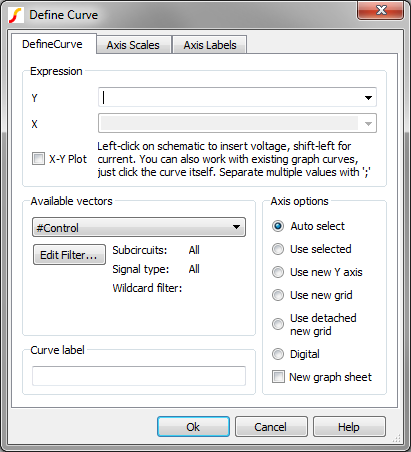
- Execute the menu bar Probe ▶ Fourier ▶
Arbitrary...Result: the Define Fourier Plot Dialog opens:
Discussion
A detailed treatment of the Fourier techniques that are only briefly touched upon in this topic could easily fill a book as the Fourier methods are, by their very nature, extremely complex. Therefore, this topic will focus more on how to generate the curves rather than the details of the Fourier techniques.
SIMetrix/SIMPLIS has two binary Fourier functions built-into the program. The functions are:
- Fourier() - this function calculates a continuous Fourier transform of the time-domain data. It uses an integration technique, and is therefore susceptible to errors caused by excessively large time steps.
- FFT() - calculates the discrete Fourier transform of the time domain data. This function requires the data to be evenly spaced with the number of plot points equal to a power of 2. This approach is susceptible to aliasing.
While the functions are available for general use, there is a dialog function similar to the Define Curve Dialog covered in topic 2.4.3 Defining Arbitrary Curves which aids in the plotting of a frequency spectrum. The dialog can be accessed from the menu bar Probe ▶ Fourier ▶ Arbitrary...
Exercise #2: Plotting the Frequency Spectrum Using the Define Fourier Plot Dialog
In this exercise, you will plot the frequency spectrum of the power supply input current. This is the current in the source V1.
- First, you need to select the vector for which you want the frequency spectrum. To define the curve vector, select the Define Curve tab on the Define Fourier Plot Dialog.
- Move the mouse to the positive pin of the input source, V1, on the
schematic.
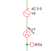
- Press and hold the shift key while left-clicking on the positive side of the
V1 source to use the input source current for the Fourier plot. Result: The Y expression is populated with the current vector V1#P.
- Click Ok. Result: The frequency spectrum for the input current is plotted on a new graph tab. The default settings will calculate the spectrum using the FFT algorithm, and the plot is on a new graph sheet because the X-axis is in Frequency, not time.
Exercise #3: The Spectrum Function
In the first exercise, the FFT was plotted using the interactive Define Fourier Plot dialog. There also exists a function which you can use to define a basic FFT plot. The Spectrum function is implemented in the SIMetrix/SIMPLIS script language, and behind the scenes, uses the FFT algorithm. It requires only two arguments:
- The vector to operate on.
- The number of interpolation points. This must be a integral power of two.
To use the Spectrum function in the Define Curve Dialog, follow these steps:
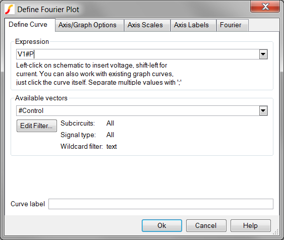
- From the menu bar, select Probe ▶ Add
Curve...
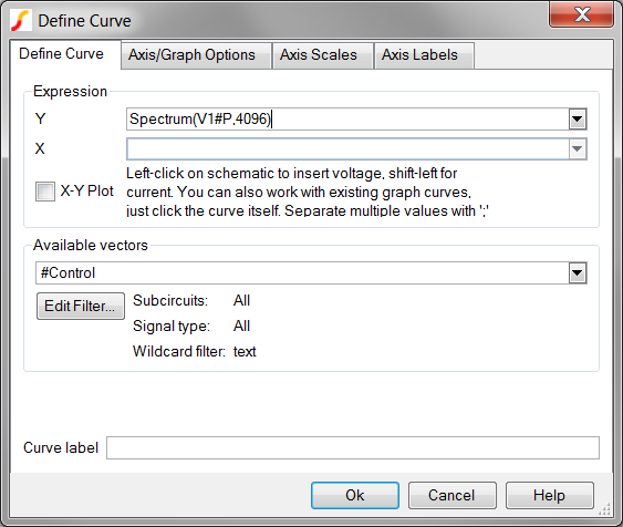
Result: The Define Curve Dialog opens:
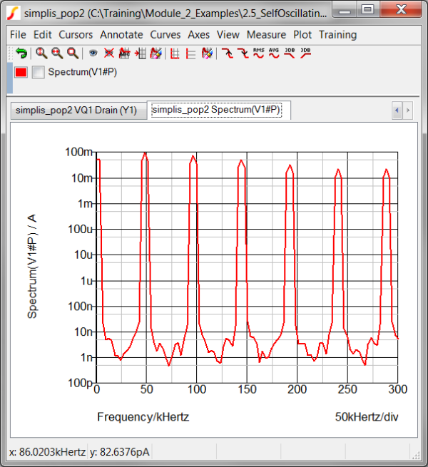
- In the Y Expression box type Spectrum(V1#P,4096). Result: The dialog should appear as follows:
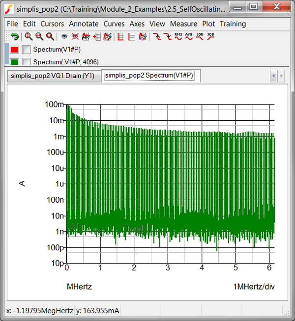
- Press Ok. Result: The spectrum is plotted on the same graph tab as you used in the last exercise. The results are identical, except the Spectrum plots the spectrum to a much higher frequency.
As you will see in topic 2.4.5 The .GRAPH Statement the Spectrum function can be used in conjunction with the .GRAPH Statement, allowing you to automatically plot the frequency spectrum of a signal after each simulation.
See also .GRAPH.
Conclusions and Key Points to Remember
- You can plot the Frequency Spectrum of any vector using the menu bar Probe ▶ Fourier▶ Arbitrary...
- The Spectrum function offers a dialog-less method for plotting frequency spectrums.