PID Discrete Time Filter
The PID Discrete Time Filter models an analog PID filter with the transfer function shown below:
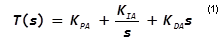
where the A in the three coefficients KPA, KIA, and KDA signifies that these coefficients are associated with Eq. (1), which is defined for the analog PID filter. For more information, see Detailed Device Operation.
The information in this topic refers to the latest PID Discrete Time Filter which was introduced in version 8.10. In versions prior to 8.10, a similar Discrete Time Filter exists and has the same behavior as the new version. The new version is implemented in a library file as opposed to a templatescript, but the electrical behavior is identical. If you require a discrete time filter for use in versions prior to 8.10, the old PID Discrete Time Filter can be placed from the part selector location: .
Related topics:
In this topic:
| Model Name: | PID Discrete Time Filter | |||
| Simulator: | This device is compatible with the SIMPLIS simulator. | |||
| Parts Selector Menu Location: | ||||
| Symbol Library: | simplis_discrete_time_filters.sxslb | |||
| Model Library: | simplis_discrete_time_filters.lb | |||
| Subcircuit Name: | SIMPLIS_DTF_PID_FILTER_Y__V2 | |||
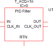
| Symbol: |
|
|||
| Multiple Selections: | Only one device at a time can be edited. | |||
Editing the PID Discrete Filter
To configure the PID Discrete Filter, follow these steps:
- Double click the symbol on the schematic to open the editing dialog to the Parameters tab.
- Make the appropriate changes to the fields described in the table below the image.
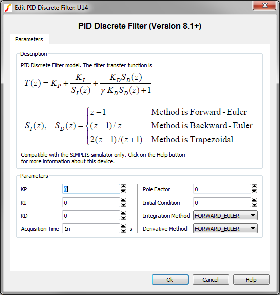
| Label | Parameter Description |
| KP | Proportional coefficient |
| KI | Integral coefficient |
| KD | Derivative coefficient |
| Acquisition Time | Filter acquisition time in seconds |
| Pole Factor | Pole factor for derivative |
| Initial Condition | Initial condition of the Discrete Time Filter output at time=0 |
| Integration Method | Integration method |
| Derivative Method | Derivative method |
Detailed Device Operation
Eq. (1), which has two zeroes and one pole, results in an improper transfer function or filter because there are more zeroes than poles. A pole is sometimes added to the derivative term to limit the bandwidth at higher frequencies. One form for such a PID filter with a pole added for the derivative action is shown below:
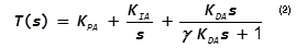
In the discrete PID filter provided, the implemented transfer function is as follows:
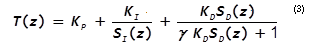
where KP, KI, and KD are coefficients entered in the dialog. To match the frequency response of the discrete PID filter represented by Eq. (3) to the frequency response of the analog PID filter represented by Eq. (2), a first-order approximation is to set KP KI and KD as follows:
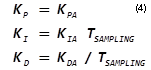
where TSAMPLING is the sampling period.
If this first-order approximation is used, the frequency response for Eq. (3) will have a good match with the frequency response for Eq. (2), as long as the poles and zeroes of Eq. (3) are more than two decades below the sampling frequency.
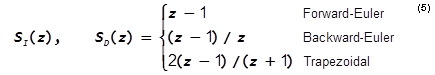
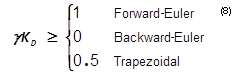
- Forward-Euler
- Backward-Euler
- Trapezoidal
If the poles and zeros of the original analog PID filter are well below the sampling frequency, then the three integration methods and the three derivative methods yield essentially the same result. These three methods are provided as a convenience if you are using one of the three mappings or transformations as a quick way to implement a discrete PID filter when the desired analog PID transfer function has been established.
The mapping functions for the three transformation methods are shown in Eq. 5:
Due to the nature of Eq. (3) and Eq. (5), the discrete PID filter has two poles in the z-domain with one from the integration term and one from the derivative term. The pole from the integration term is always located at z=1 and the pole due to the derivative term is
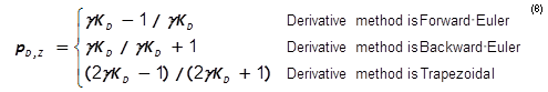
Where γ is the derivative term pole factor.
Since the location of this pole should not yield unstable responses, at the very minimum, the restraint on PD,Z is
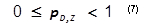
From Eq. (6) and Eq. (7), the restriction placed on the product γKD is
Once the value of PD,Z is set, γ can be computed from Eq. (6). The corresponding pole location in the s-domain for the pole PD,Z in the z-domain is
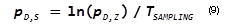
If PD,Z is set to 0.5, the corresponding pole in the s-domain would have a corner frequency of about 0.11 of the sampling frequency.
If there are already extra low-pass filters along the path of feedback, it may be desirable not to introduce the extra pole associated with the derivative term in the discrete PID filter described here.
While it is not exactly the same as removing the extra pole, placing the center of the origin of the complex plane (PD,Z) at z=0.0 has almost the same effect. Such a pole will have no effect on the magnitude of the derivative term but will introduce a phase delay to the derivative term. Such a phase delay is minimal until the signal of interest is at or above one-tenth of the sampling frequency.
In addition, if you are using one of the three mappings or transformations, the derivative method should be set to the same as the integration method. The two methods are allowed to be different here in case you do not use the mapping or transformation point of view, but, instead, implement the integration and determine the derivative from the input samples.
Examples
The test circuit used to generate the waveform examples in the next section can be downloaded here: simplis_035_piddiscretefilter_example.sxsch.
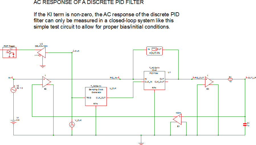
Waveforms
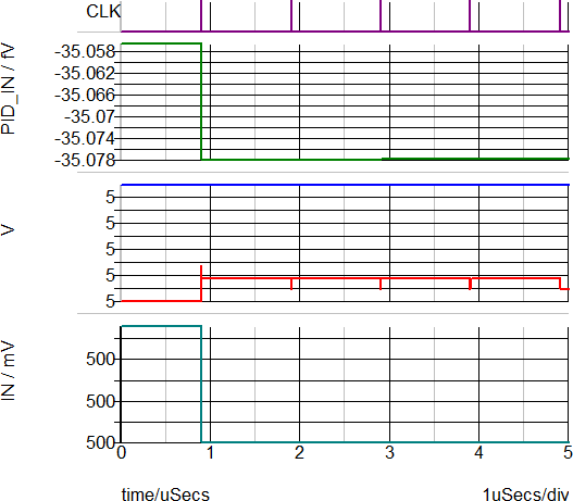
The POP waveforms below show the steady state operation of the PID filter. The PID input, PID_IN , is forced to nearly zero by the external feedback components and the high integral gain of the PID Filter. The middle grid has both the PID_OUT and OUT_LP curves, and both are at the steady state voltages of 5V. The bottom-most curve representing the input voltage, IN , is at the DC setpoint of 0.5V.
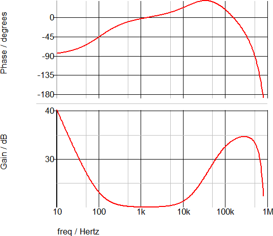
The following AC waveforms plot the gain and phase of the PID discrete time filter. The gain at low frequency is dominated by the integral portion of the filter, followed by a proportional gain of approximately 20dB.
Subcircuit Parameters
The subcircuit parameter names, data types, ranges, units, and descriptions are in the following table. The parameter names can be used to generate netlist entries for the device. For example, a valid PID Discrete Time Filter netlist entry would be:
X$U1 19 23 0 22 0 SIMPLIS_DTF_PID_FILTER_Y__V2 vars: IC=0 DERIVATIVE_METHOD='FORWARD_EULER' GAMMA=0 INTEGRATION_METHOD='FORWARD_EULER' KD=0 KI=0 KP=0 T_ACQ=1n
| Parameter Name | Label | Data Type | Range | Units | Parameter Description |
| DERIVATIVE_METHOD | Derivative Method | String |
|
none | Derivative method |
| GAMMA | Pole Factor | Number | any | none | Pole factor for derivative |
| IC | Initial Condition | Number |
|
none | Initial condition of the Discrete Time Filter output at time=0 |
| INTEGRATION_METHOD | Integration Method | String |
|
none | Integration method |
| KD | KD | Number | any | none | Derivative coefficient |
| KI | KI | Number | any | none | Integral coefficient |
| KP | KP | Number | any | none | Proportional coefficient |
| T_ACQ | Acquisition Time | Number | min: 1f | s | Filter acquisition time in seconds |